LINEAR SYSTEMS

By John Gilbert

Extending to ${\mathbb R}^n$ the equation $a x + by = c$ of a line in ${\mathbb R}^2$ and a plane $Ax + By + Cz = D$ in ${\mathbb R}^3$ we arrive at

Definition 3.1: a LINEAR EQUATION in $n$ variables $x_1, \, x_2, \, \ldots,\, x_{n}$ is an equation of the form $$a_1 x_1 + a_2 x_2 + \ldots a_{n} x_{n} \ = \ b$$ where the COEFFICIENTS $a_1,\, a_2, \, \ldots,\, a_{n}$ and CONSTANT TERM $b$ are real numbers.

A SOLUTION of this equation is a vector ${\bf x}$ in ${\mathbb R}^n$ whose components $s_1,\, s_2,\, \ldots,\, s_{n}$ satisfy the equation when we substitute $x_1 = s_1,\, x_2 = s_2,\, \ldots,\, x_{n} = s_{n}$.

By a Linear System of $m$ algebraic equations in $n$ variables we mean the set of $m$ linear equations: $$\begin{array}{cc} a_{11} x_1 + a_{12} x_2 + \cdots + a_{1,\,n} x_{n} & = & b_1\\ a_{21} x_1 + a_{22} x_2 + \cdots + a_{2,\, n} x_{n} & = & b_2\\ & \vdots & \\ a_{m,\, 1} x_1 + a_{m,\,2} x_2 + \cdots + a_{m,\,n} x_{n} & = & b_{m} \end{array}$$

Lines and planes provide geometric illustrations of linear systems. Here is some important terminology for linear systems:

a Solution for the system consists of a vector ${\bf x}$ in ${\mathbb R}^n$ that is a simultaneous solution of each equation,

the set of all solutions is called, not surprisingly, the Solution Set of the system,

two systems of linear equations are said to be Equivalent when they have the same solution set.

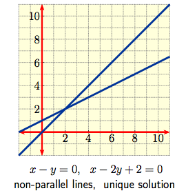
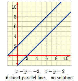
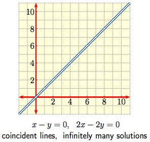
The case $m = n = 2$ becomes a pair of simultaneous linear equations $$a_{11} x + a_{12} y \ = \ b_1\,, \qquad \qquad a_{21} x + a_{22} y \ = \ b_2\,, $$ in $2$ variables which can be thought of graphically as a pair of straight lines in the plane. The solution set then consists of the point(s) of intersection, if any, of the lines. The various possibilities are shown in:

The first system has a unique solution because the lines intersect in a single point. In the second and third examples, however, the lines are parallel, so the solution set will be empty when the parallel lines are distinct as in the second example, while the system will have infinitely many solutions when the parallel lines coincide as in the third case. So for a general system one can also ask

Fundamental Questions: for a general system of linear equations:

Is the system CONSISTENT, i.e., does there exist at least one solution?

If a solution exists, is it the only one, i.e, is it UNIQUE?

If there is more than one solution, are there INFINITELY MANY solutions?

If no solution exists, i.e., the solution set is empty, we say the system is INCONSISTENT.

In dimensions $2$ and $3$ it is thus clear geometrically that the system is inconsistent or consistent and had either one or infinitely many solutions. Seeking answers beyond $3$ variables, however, requires all the linear algebra we've set in place! To each system of $m$ linear equations in $n$ variables we associate two matrices:

1. Coefficient matrix: the coefficients are written as rows with entries aligned so that a column consists of the coefficients of an individual variable: $$\left[\begin{array}{cc} a_{11} & a_{12} & a_{12} & \cdots & a_{1,\, n} \\ a_{21} & a_{22} & a_{22} & \cdots & a_{2,\, n} \\ \vdots & \vdots & \vdots & \ddots & \vdots \\ a_{m,\, 1} & a_{m,\, 2} & a_{m,\, 2} & \cdots & a_{m,\, n} \end{array}\right]\,$$ making an $m \times n$ matrix.

2. Augmented matrix: now augment the coefficient matrix by adding the column of constant terms to the $n$ columns of the coefficient matrix: $$\left[\begin{array}{cc} a_{11} & a_{12} & a_{12} & \cdots & a_{1,\, n} & b_1\\ a_{21} & a_{22} & a_{22} & \cdots & a_{2,\, n} & b_2\\ \vdots & \vdots & \vdots & \ddots & \vdots & \vdots \\ a_{m,\,1} & a_{m,\, 2} & a_{m,\, 2} & \cdots & a_{m,\, n} & b_{m} \end{array}\right]\,$$ making an $m \times (n+1)$ matrix.

Since any matrix with $m$ rows can be written as a row of column vectors in ${\mathbb R}^m$, set

$$ {\bf a}_1 \ = \ \left[\begin{array}{cc} a_{11} \\ a_{21} \\ \vdots \\ a_{m,\, 1} \end{array} \right], \qquad {\bf a}_2 \ = \ \left[\begin{array}{cc} a_{12} \\ a_{22} \\ \vdots \\ a_{m,\,2} \end{array} \right], \quad \ldots \quad {\bf a}_{n} \ = \ \left[\begin{array}{cc} a_{1,\, n} \\ a_{2,\, n} \\ \vdots \\ a_{m,\, n} \end{array} \right], \qquad {\bf b} \ = \ \left[\begin{array}{cc} b_1 \\ b_2 \\ \vdots \\ b_{m} \end{array} \right].$$ Then the coefficient and augmented matrices can be re-written as $$ A \ = \ \left[ {\bf a}_1 \ \ {\bf a}_2 \ \ \dots \ \ {\bf a}_{n} \right], \qquad \qquad [A \ \ {\bf b}] \ = \ \left[ {\bf a}_1 \ \ {\bf a}_2 \ \ \dots \ \ {\bf a}_{n} \ \ {\bf b}\right]. $$ On the other hand, by scalar multiplication and addition of vectors as well as the matrix-vector rule, $$ x_1 {\bf a}_1 + x_2 {\bf a}_2 + \cdots + x_{n}{\bf a}_{n} \ = \ \left[\begin{array}{cc} a_{11} x_1 + a_{12} x_2 + \cdots + a_{1,\, n} x_{n} \\ a_{21} x_1 + a_{22} x_2 + \cdots + a_{2,\, n} x_{n} \\ \vdots \\ a_{m,\, 1} x_1 + a_{m,2} x_2 + \cdots + a_{m,\, n} \end{array}\right] \ = \ A \left[\begin{array}{cc} x_1 \\ x_2 \\ \vdots \\ x_{n}\end{array} \right] \ = \ A {\bf x} \,. $$ So a general system of $m$ linear equations in $n$ variables can be re-interpreted in three different ways:

$ \qquad \qquad \qquad \qquad \quad [A \ \ {\bf b}] \qquad \qquad \qquad \qquad \qquad \qquad $ an augmented matrix,

$ \qquad \qquad x_1 {\bf a}_1 + x_2 {\bf a}_2 + \ldots + x_{n}{\bf a}_{n} \ = \ {\bf b} \qquad \qquad \qquad \qquad $ a vector equation,

$ \qquad \qquad \qquad \qquad A {\bf x} \ = {\bf b}\qquad \qquad \qquad \qquad \qquad \qquad \ $ a matrix equation.

Thus a vector ${\bf x}$ in ${\mathbb R}^n$ will be a solution of the system of linear equations if and only it is a solution of the vector equation, and in turn if and only if it is a solution of the matrix equation, proving

Fundamental Theorem 3.1: if ${\bf a}_1, \,{\bf a}_2,\, \ldots,\, {\bf a}_{n}$ and ${\bf b}$ are vectors in ${\mathbb R}^m$, then each of the following
   the system of linear equations with augmented matrix $\left[\begin{array}{cc} \,{\bf a}_1 & {\bf a}_2 & \cdots & {\bf a}_{n} & {\bf b}\,\\ \end{array}\right]\, $,

   the vector equation $x_1 {\bf a}_1\, + \,x_2 {\bf a}_2\, +\, \cdots\, +\, x_{n} {\bf a}_{n} \ = \ {\bf b}\,$,

   the matrix equation $A{\bf x} = {\bf b}\,$ with $A=\left[\begin{array}{cc} \,{\bf a}_1 & {\bf a}_2 & \cdots & {\bf a}_{n} \\ \end{array}\right]\, $ ,
has the same solution set.

This is a huge result conceptually and computationally! In practice, a system may consist of hundreds or thousands (millions?) of equations and variables, yet the system has been re-interpreted in as simple a form as the equations $a_1 x + a_2 y = b$ or $a x = b$ you studied in high school, irrespective of the size of $m$ and $n$. More significantly from a computational point of view, the augmented matrix is simply a list of lists - something a computer can understand - so perhaps efficient algorithms can be developed by transcribing for matrices the elimination of variable idea used earlier. We display the algebraic steps side-by-side with the corresponding row operations on augmented matrices.

Problem 3.1: solve for $x,\,y$ in the system $$ \begin{array}{cc}(1) \ \ \qquad ax + by \,=\, r \qquad \qquad \qquad \\ (2) \qquad c x + d y \,=\, s \qquad \qquad \qquad \end{array}$$

Algebraic Solution: So long as $a \ne 0$, we can subtract $\frac{c}{a}$ times equation $(1)$ from equation $(2)$ to eliminate $x$ from equation $(2)$ giving a new system: $$ \begin{array}{cc}(1) \qquad \quad \quad ax + by \,=\, r \qquad \qquad \qquad \qquad \\ (2)\quad \ 0 x +\textstyle{\frac{1}{a}}(ad - bc) y \,=\, \textstyle{\frac{1}{a}}(a s -c r) \qquad \qquad\end{array}$$ with the same solution set. Now use (2) to solve for $y$: $$\qquad y \ = \ \frac{a s - c r}{a d - b c}\,, \qquad \text{if}\ \ ad - bc \ne 0,$$ and then $x$ can be found by substituting back for $y$ in (1): $$x \,=\, \frac {r d - bs}{a d - b c}, \qquad y \,=\, \frac{a s - c r}{a d - b c}\,.$$

Matrix Solution: the corresponding augmented matrix is $$ \left[\begin{array}{cc} a & b & r \\ c & d & s \end{array}\right] .$$ Subtract $\frac{c}{a}$Row 1 from Row 2 to create a new Row 2: $$ \xrightarrow{ R_2 - \frac{c}{a}R_1 } \ \left[\begin{array}{cc} a & b & r \\ 0 & \textstyle{\frac{1}{a}}(ad - bc) & \textstyle{\frac{1}{a}}(a s -c r) \end{array}\right]\,. $$ This is the augmented matrix associated with the linear system to the left. Crucially,

the row operation did not change the solution set,

the new augmented matrix is in ECHELON FORM,

from which solutions $x,\,y$ can be read off quickly by back substitution.

So the basic idea is to perform row operations to reduce the augmented matrix to a matrix in ECHELON FORM corresponding to an EQUIVALENT linear system.

Problem 3.2: solve for $x, \, y$ and $z$ in the system $$\begin{array}{cc} \phantom{\ \quad \quad} y +z & = & 4\,, \\ 3x + 6y -3z & = & 3\,, \\ -2x -3y + 7z & = & 10\,.\end{array} $$

Matrix Solution: The associated augmented matrix is $$[ A\ \ {\bf b}] \ = \ \left[\begin{array}{cc} 0 & 1 & 1 & 4 \\ 3 & 6 & -3 & 3 \\ -2 & -3 & 7 & 10\end{array} \right]. $$ Since the first entry in the first row of $[ A\ \ {\bf b}]$ is $0$, interchange Row 1 and Row 2: $$[ A \ \ {\bf b}] \ \xrightarrow{ R_1\, \leftrightarrow \, R_2 } \ \left[\begin{array}{cc} 3 & 6 & -3 & 3 \\ 0 & 1 & 1 & 4 \\ -2 & -3 & 7 & 10\end{array} \right]. $$ To simplify calculations mutiply the new Row 1 by $1/3$: $$ \xrightarrow{ \frac{1}{3}R_1 \, \rightarrow \, R_1 } \ \left[\begin{array}{cc} 1 & 2 & -1 & 1 \\ 0 & 1 & 1 & 4 \\ -2 & -3 & 7 & 10\end{array} \right]. $$

Now as before we can successively add/subtract multiples of one row to another to introduce 0 entries: $$ \xrightarrow{ R_3 +2 R_1 \rightarrow R_3 } \ \left[\begin{array}{cc} 1 & 2 & -1 & 1 \\ 0 & 1 & 1 & 4 \\ 0 & 1 & 5 & 12\end{array} \right] $$ $$ \xrightarrow{ R_3 - R_2 \rightarrow R_3 } \ \left[\begin{array}{cc} 1 & 2 & -1 & 1 \\ 0 & 1 & 1 & 4 \\ 0 & 0 & 4 & 8\end{array} \right], $$ which is the augmented matrix associated with the equivalent system $$\begin{array}{cc} x + 2y -z & = & 1\,, \\ \phantom{\ \ \quad \quad} y +z & = & 4\,, \\ \phantom{ \qquad \qquad} 4z & = & 8\,.\end{array} $$ Thus $z = 2$, and hence $ y = 2,\ \ x \,=\,-1$ by back substitution.

Wasn't that simpler and more systematic than going through the tedious algebraic details for systems of equations!

Solving systems of linear equations by reducing the corresponding augmented matrix to 'Echelon' form applies quite generally. It is usually known as Gaussian Elimination because of its use by Gauss in the early 19th century, though it was known many years earlier to the Chinese. In fact, the same operations as before, now called Elementary Row operations, can be carried out on the rows of any matrix, whatever the size. Formally,

Elementary Row Operations on a matrix:

(Interchange) interchange two rows,

(Scaling) multiply all entries in a row by a non-zero constant,

(Replacement) replace one row by the sum of itself and a multiple of another row.

We shall say that matrices $A,\, B$ are Row Equivalent, and write $A \, \sim \, B$, when there is a sequence of elementary row operations that takes $A$ into $B$. For later purposes, note also that elementary row operations are reversible, so if $A\, \sim \, B$, then $B \, \sim \, A$.

But the crucial echelon form that simplified solving the system in $2$ and $3$ variables carries over to general systems: the earlier examples of

$$ \left[\begin{array}{cc} a & b & r \\ 0 & \textstyle{\frac{1}{a}}(ad - bc) & {\phantom{u \over v}\!\!\!} \textstyle{\frac{1}{a}}(a s -c r) \end{array}\right], \qquad \qquad \left[\begin{array}{cc} 1 & 2 & -1 & 1 \\ 0 & 1 & 1 & 4 \\ 0 & 0 & 4 & 8\end{array} \right] $$ suggest the following:

Definition 3.2: a matrix is said to be in (Row) Echelon Form if
all non-zero rows lie above any row of all zeros,

for each non-zero row, the leading entry, i.e., the left-most non-zero entry, lies in a column to the left of any leading entry below it.

In particular, in any column containing a leading entry all entries below that leading entry are zero. Thus

$$\left[\begin{array}{cc} \circledast & \ast & \ast & \ast & \ast & \ast & \ast & \cdots & \ast \\ 0 & 0 & \circledast & \ast & \ast & \ast & \ast & \cdots & \ast \\ 0 & 0 & 0 & \circledast & \ast & \ast & \ast & \cdots & \ast \\ 0 & 0 & 0 & 0 & 0 & \circledast & \ast & \cdots & \ast\\ 0 & 0 & 0 & 0 & 0 & 0 & 0 & \cdots & 0 \\ 0 & 0 & 0 & 0 & 0 & 0 & 0 & \cdots & 0 \end{array}\right], \qquad \qquad \left[\begin{array}{cc} 0 &\circledast & \ast & \ast & \ast & \ast & \ast & \cdots & \ast \\ 0 & 0 & \circledast & \ast & \ast & \ast & \ast & \cdots & \ast \\ 0 & 0 & 0 & 0 & \circledast & \ast & \ast & \cdots & \ast \\ 0 & 0 & 0 & 0 & 0 & \circledast & \ast & \cdots & \ast\\ 0 & 0 & 0 & 0 & 0 & 0 & 0 & \cdots & 0 \\ 0 & 0 & 0 & 0 & 0 & 0 & 0 & \cdots & 0 \end{array}\right],$$

are typical structures for a general matrix in Row Echelon Form; the $\circledast$ entry in a non-zero row is the leading entry, often called a pivot, and all $\ast$ entries following the pivot in the row can be zero or non-zero. Columns in which a pivot $\circledast$ occurs are often called pivot columns. The terms pivot and pivot column are used because in the earlier examples of linear systems the pivots and pivot columns are what we used to row reduce the augmented matrix to echelon form (we "pivoted around them"). Each matrix is row equivalent to a matrix in echelon form. Let's investigate how reducing a matrix to echelon form helps solving linear systems. The first example simply makes a slight change in the third equations in 3.2:

Problem 3.3: solve for $x,\, y$ and $z$ in

$$\begin{array}{cc} \phantom{\ \quad \quad} y +z & = & 4\,, \\ 3x + 6y -3z & = & 3\,, \\ -2x -3y + 3z & = & 10\,.\end{array} $$

Solution: the associated augmented matrix now is $$[ A \ \ {\bf b}] \ = \ \left[\begin{array}{cc} 0 & 1 & 1 & 4 \\ 3 & 6 & -3 & 3 \\ -2 & -3 & 3 & 10\end{array} \right], $$ and by the same row reductions as before we obtain a row equivalent echelon form

$$[ A \ \ {\bf b}] \ \sim \ \left[\begin{array}{cc} 1 & 2 & -1 & 1 \\ 0 & 1 & 1 & 4 \\ 0 & 0 & 0 & 1\end{array} \right] \ (\ = \ B, \ \text{say},\,), $$ associated with the equivalent system $$\begin{array}{cc} x +2y - z & = & 1\,, \\ \phantom{\ \ \qquad } y +z & = & 4\,, \\ \phantom{ \qquad \qquad} 0z & = & 1\,.\end{array} $$ But now there is no value of $z$ such that $0 z = 1$, so the system is Inconsistent. We can see this from the echelon form $B$: it has three pivot columns, but the column of right hand sides is one of them!!

Existence Theorem 3.2: a linear system is Consistent if and only if an echelon form of the associated augmented matrix has NO row of the form $$[\, 0 \ \ 0 \ \ \ldots \ \ 0 \ \ b\,]\,, \qquad b \ \ne 0\,.$$

Time now to begin investigating questions of Uniqueness or Infinitely many solutions for systems. Problem 3.3 simply repeats Problem 3.2, while the Problem 3.5 modifies the third equation in Problem 3.3.

Problem 3.4: solve for $x,\, y$ and $z$ in $$\begin{array}{cc} \phantom{\ \quad \quad} y +z & = & 4\,, \\ 3x + 6y -3z & = & 3\,, \\ -2x -3y + 7z & = & 10\,.\end{array} $$

Solution: the associated augmented matrix is $$[ A \ \ {\bf b}] \ = \ \left[\begin{array}{cc} 0 & 1 & 1 & 4 \\ 3 & 6 & -3 & 3 \\ -2 & -3 & 7 & 10\end{array} \right], $$ and by the same row reductions as before, we obtain a row equivalent echelon form

$$[ A \ \ {\bf b}] \ \sim \left[\begin{array}{cc} 1 & 2 & -1 & 1 \\ 0 & 1 & 1 & 4 \\ 0 & 0 & 4 & 8\end{array} \right] \ (\ = \ B, \ \text{say},\,) $$ associated with the equivalent system $$\begin{array}{cc} x + 2y -z & = & 1\,, \\ \phantom{\ \ \quad \quad} y +z & = & 4\,, \\ \phantom{ \qquad \qquad} 4z & = & 8\,.\end{array} $$ By Theorem 3.2, the system is consistent. Unique solutions $$z\,=\, 2,\quad y\,=\,2,\quad x\,=\, -1$$ are easily calculated directly and by back substitution.

Problem 3.5: solve for $x,\, y$ and $z$ in

$$\begin{array}{cc} \phantom{\ \quad \quad} y +z & = & 4\,, \\ 3x + 6y -3z & = & 3\,, \\ -2x -3y + 3z & = & 2\,.\end{array} $$

Solution: the associated augmented matrix is $$[ A\ \ {\bf b}] \ = \ \left[\begin{array}{cc} 0 & 1 & 1 & 4 \\ 3 & 6 & -3 & 3 \\ -2 & -3 & 3 & 2\end{array} \right], $$ and by the same row reductions as before, we obtain a row equivalent echelon form

$$[ A\ \ {\bf b}]\ \sim \ \left[\begin{array}{cc} 1 & 2 & -1 & 1 \\ 0 & 1 & 1 & 4 \\ 0 & 0 & 0 & 0\end{array} \right] \quad (= B \ \text{say}) $$ associated with the equivalent system $$\begin{array}{cc} x +2 y -z & = & 1\,, \\ \phantom{\ \ \quad } y +z & = & 4\,.\end{array} $$ Now there is no equation to specify $z$, so $z$ is a free variable: $$\quad x \,=\, 3 t-7\,, \quad y \,=\, 4-t\,, \quad z \,=\, t\,, \ \ (t \ \text{arbitrary}).$$ This can also be seen from $B$: only the $x$- and $y$-columns are pivot columns.

The examples just gone through thus provide the first of the algorithms for solving general systems of linear equations:

Gauss Elimination: given a general system of $m$ linear equations in $n$ variables,

form the associated augmented matrix $[ A\ \ {\bf b}]$ and compute an echelon form $B$,

if the right hand-most column of $B$ is a pivot column, then the system is inconsistent, otherwise the system is consistent,

if the system is consistent, then any variable corresponding to a pivot column is called a dependent variable, otherwise the variable is called a free variable.

You will usually be asked to give the solution to a linear system in Vector Form:

Vector Form: Given a linear system with associated matrix equation $A{\bf x} = {\bf b}\,$ and free variables $r_1, \dots , r_k$, the solution set can be written as a linear combination $${\bf x} \ = \ {\bf v}_0 + r_1 {\bf v}_1 + \cdots + r_k {\bf v}_k$$ with ${\bf v}_0 , \dots , {\bf v}_k \in \mathbb{R}^n$.

In Problem 3.4, the Vector Form of the solution is $${\bf x} \ = \ \left[\begin{array}{cc} -1 \cr 2 \cr 2 \end{array}\right].$$

In Problem 3.5, the Vector Form of the solution is $${\bf x} \ = \ \left[\begin{array}{cc} 3t-7 \cr 4-t \cr t \end{array}\right] \ = \ \left[\begin{array}{cc} -7 \cr 4 \cr 0 \end{array}\right] + t \, \left[\begin{array}{cc} 3 \cr -1 \cr 1 \end{array}\right].$$

A typical geometric application is the following.

Problem 3.6: express the plane ${\cal P}$ in ${\mathbb R}^3$ given in vector form by $${\bf x} \ = \ \left[\begin{array}{cc} 2 \cr -1 \cr 2 \end{array}\right] +s\,\left[\begin{array}{cc} 1 \cr 1 \cr 2 \end{array}\right] +t\,\left[\begin{array}{cc} -3 \cr -5 \cr -8 \end{array}\right], $$ as a linear equation in $x,\, y$ and $z$.

Solution: a vector ${\bf x}$ in ${\mathbb R}^3$ lies in ${\cal P}$ when $$\left[\begin{array}{cc} x \cr y \cr z \end{array}\right] \ = \ \left[\begin{array}{cc} 2 \cr -1 \cr 2 \end{array}\right] +s\,\left[\begin{array}{cc} 1 \cr 1 \cr 2 \end{array}\right] +t\,\left[\begin{array}{cc} -3 \cr -5 \cr -8 \end{array}\right], $$ for some choice of $s,\, t$, i.e., when $$ s\,\left[\begin{array}{cc} 1 \cr 1 \cr 2 \end{array}\right] +t\,\left[\begin{array}{cc} -3 \cr -5 \cr -8 \end{array}\right] \ = \ \left[\begin{array}{cc} x-2 \cr y+1 \cr z-2 \end{array}\right]$$ is consistent as a vector equation in $s,\, t$. The associated augmented matrix is

$$[ A\ \ {\bf b}] \ = \ \left[\begin{array}{cc} 1 & -3 & x-2 \\ 1 & -5 & y+1 \\ 2 & -8 & z-2\end{array} \right]. $$

Now by row reduction in the first column of $[ A\ \ {\bf b}]$, we obtain $$[ A\ \ {\bf b}]\ \sim \ \left[\begin{array}{cc} 1 & -3 & x-2 \\ 0 & -2 & y-x+3 \\ 0 & -2 & z - 2x +2 \end{array}\right],$$ and after row reduction in the second column, $$[ A\ \ {\bf b}]\ \sim \ \left[\begin{array}{cc} 1 & -3 & x-2 \\ 0 & -2 & y-x+3 \\ 0 & 0 & z - x-y -1 \end{array}\right].$$ But by Existence Theorem 3.2, the vector equation will be consistent if and only if the right hand-most column is not a pivot column, i.e. when $$z - x - y - 1 \ = \ 0\,. $$