A Predator-Prey model:

Suppose that we have two populations, one of which eats the other. For instance, you might imagine owls and mice, or wolves and elk. Let $P(t)$ be the number of prey at time $t$, and $L(t)$ the number of predators. We wish to understand the interaction between the two populations.

The rate at which the predators eat the prey is proportional to how often a predator meets a prey, i.e. to the product $P(t)L(t)$ of the predator population and the prey population. This adds to the predator population (since it means extra food) and subtracts from the prey population (since they get eaten).

For the prey, we will use our logistic growth model but now we will include an additional term that accounts for some of them getting killed by predators. That is, $$P' = rP(1 -P/K) - cPL, \qquad P(0) = P_0.$$ For the predators, we assume the growth of their population is proportional to the number of prey consumed ($dPL$), and that they die off at a rate proportional to their population ($eL$). These assumptions lead to the equation $$L' = dPL- eL, \qquad L(0) = L_0.$$ This coupled predator-prey model is called the Lotka-Volterra model with bounded growth, and involves five parameters and two initial conditions:

1. The reproduction rate $r$ of the prey.
2. The carrying capacity $K$ of the prey in the absence of predators
3. A constant $c$ that describes how much encounters between predators and prey tend to deplete the population of prey.
4. A constant $d$ that describes how much these encounters help the predator population, and
5. A constant $e$ that describes how quickly the predator population would die off in the absence of prey.
6. The initial population $P_0$ of prey, and
7. The initial population $L_0$ of predators.

To investigate the behavior of this model, we will use MATLAB's ODE solver. Please open MATLAB yourself and play around with this. See how changing the parameters affects the solution. The m-file (with a particular set of parameter values) and the needed commands are shown below.   

line 1   %This function is used for solving the SIR model numerically using ode45.

line 2   %It contains the information with regard to the system of equations.

line 3   function LVequ = PPsys(t,pp)

line 4   r = 0.1; %this is the parameter value for r

line 5   K = 10000; %this is the parameter value for K

line 6   c = 0.005; %this is the parameter value for c

line 7   d = .00004; %this is the parameter value for d

line 8   e = 0.04; %this is the parameter value for e

line 9   LVequ = [r*pp(1)*(1 - pp(1)/K) - c*pp(1)*pp(2); d*pp(1)*pp(2) - pp(2)*e];

line 10 %LVequ is a vector that contains the Lotka-Volterra differential equations

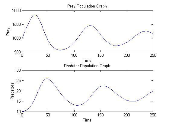
Assume initial population of 10 and 1000 for the predator and prey, respectively, we can now numerically solve this system.  In the Matlab Command Window enter

>>  [t,pp]=ode45('PPsys',[0,250],[1000,10]);

>>  figure

>>  subplot(2,1,1);

>>  plot(t,pp(:,1));

>> title('Prey Population Graph'), ylabel('Prey'), xlabel('Time')

>> subplot(2,1,2);

>> plot(t,pp(:,2));

>> title('Predator Population Graph'), ylabel('Predators'), xlabel('Time')

Notice how both the predator and prey populations both oscillate, with a period of about 105 time units, and how they are not in sync. Rather, they are a quarter cycle apart. Increases in the prey population (peaking at time 25) cause the predator population to increase (peaking at time 50), which causes the prey population to drop (bottoming out at time 75 or so), which causes the predator population to drop (bottoming out around time 105), which allows the prey population to shoot back up, peaking around time 130, after which the cycle repeats again, although with lower peaks and higher troughs.

The system will eventually settle into a steady state, with an intermediate number of predators and an intermediate number of prey. However, if any external factors (like a drought or fire or harsh winter or human intervention) upset the balance, the oscillations will start back up.