Now that we know what double integrals are, we can start to compute them. The key idea is: One variable at a time!
In order to integrate over a rectangle $[a,b] \times [c,d]$, we first integrate over one variable (say, $y$) for each fixed value of $x$. That's an ordinary integral, which we can do using the fundamental theorem of calculus. We then integrate the result over the other variable (in this case $x$), which we can also do using the fundamental theorem of calculus. So a 2-dimensional double integral boils down to two ordinary 1-dimensional integrals, one inside the other. We call this an iterated integral.
There are two ways to see the relation between double integrals and iterated integrals. In the bottom-up approach, we evaluate the sum $$\sum_{i=1}^m \sum_{j=1}^n f\left(x_{i}^*,y_{j}^*\right) \,\Delta x\, \Delta y,$$ by first summing over all of the boxes with a fixed $i$ to get the contribution of a column, and then adding up the columns. (Or we can sum over all of the boxes with a fixed $j$ to get the contribution of a row, and then add up the rows.)
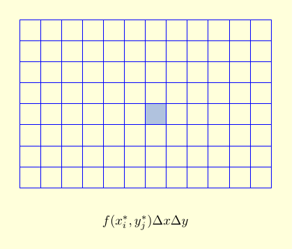
| $f\left(x_{i}^*,y_{j}^*\right)\, \Delta y\, \Delta x$ is the approximate contribution of a single box to our double integral. |
|
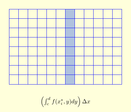
| $\displaystyle\sum_{j=1}^n f\left(x_{i}^*,y_{j}^*\right) \,\Delta y\, \Delta x$ is the approximate contribution of all the boxes in a single column. As $n \to \infty$, the sum over $n$ turns into an integral, and we get $$\displaystyle\left (\int_c^d f\left(x_i^*, y\right)\,dy \right )\, \Delta x.$$ |
|
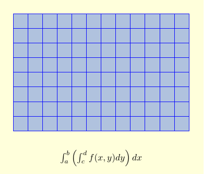
| Adding up the columns then gives $\displaystyle\sum_{i=1}^m \left (\int_c^d f\left(x_i^*, y\right)\, dy \right )\, \Delta x$. Taking a limit as $m \to \infty$ turns the sum into an iterated integral: $$\int_a^b \left ( \int_c^d f(x,y)\, dy \right ) \,dx.$$ |
|
This bottom-up approach is explained in the following video. (Video Fix? However, there is a small error. At the beginning it says that we're going to integrate over the rectangle $[0,1] \times [0,2]$, but for the rest of the video the region $R$ is actually the rectangle $[0,2] \times [0,1]$.)
An alternate approach to finding volumes (and hence double integrals)
- the so-called Slice Method - was formulated by
Cavalieri
and is expressed mathematically in
Cavalieri's Principle: let $W$ be a solid and $P_x,\, a \le x \le b,$ be a family of parallel planes such that
|
|
Example: Find the volume of the solid $W$ under the
hyperbolic paraboloid
$$z \ = \ f(x,\, y) \ = \ 2+ x^2 - y^2 $$
and over the square $D\,= \,[-1,\,1]\,\times\,[-1,\,1]$.
Solution: The solid is shown below. When $P_x$ is the vertical slice perpendicular to the $x$-axis for fixed $x$ shown in purple, then $$A(x) =\int_{-1}^2\, (2+x^2 - y^2)\, dy\qquad \qquad$$ $$\qquad = \left[\,2y +x^2y -\frac{y^3}{3}\right]_{-1}^1= \frac{10}{3} +2x^2 \,.$$ But then by using the slider to fill out the solid, Cavalieri's Principle shows that $W$ has $$\hbox{volume} \ = \ \int_{-1}^1\, A(x)\, dx \ = \ \int_{-1}^1\, \left(\frac{10}{3} +2x^2\right)\,dx \ = \ \left[\frac{10x}{3} +\frac{2x^3}{3}\right]_{-1}^1 \ = \ 8\,.$$ |
In other words, the volume of a region is $\int_a^b A(x)\, dx$, where $A(x)$ is the cross-sectional area at a particular value of $x$. But that's the area under the curve $z=f(x,y)$, where we are treating $x$ as a constant and $y$ as our variable. That is,
| The double integral $\displaystyle\iint_R f(x,y)\, dA$ equals the iterated integral $\displaystyle\int_a^b \left (\int_c^d f(x,y) \,dy\right )\, dx$. |