COMMON MISTEAKS MISTAKES IN
USING STATISTICS: Spotting and Avoiding Them
Random Variables and Probability
Distributions
I. In most applications, a random variable
can be thought of as a variable that depends on a random process. Here
are some examples to help explain the concepts involved:
1. Toss a die and look at what number is on the side that lands up.
Tossing the die is an example
of a random process; the number on top is the random variable.
2. Toss two dice and take the sum of the numbers that land up.
Tossing the dice is the
random process; the sum is the random variable.
3. Toss two dice and take the product of the numbers that land up.
Tossing the dice is the
random process; the product is the random variable.
Examples 2 and 3 together show that the same random process can be involved in
two different random variables.
4. Randomly pick (in a way that gives each student an equal
chance of being chosen) a UT student and measure their height.
Picking the student is the
random process; their height is the random variable.
5. Randomly pick (in a way that gives each student an equal chance of
being chosen) a student in a particular class and measure their height.
Picking the student is the
random process; their height is the random variable.
Examples 4 and 5 illustrate that using the same variable (in this
case, height) but different random
processes (in this case, choosing from different populations) gives different random variables.
6. Measure the height of the third student who walks into
this class.
In all the examples before
this one, the random process was done deliberately; in Example 6, the
random process is one that occurs naturally.1
Because Examples 5 and 6
involved different random processes, they are different random
variables.
7. Toss a coin and see whether it comes up heads or tails.
Tossing the coin is the
random process; the variable is heads or tails.
Example 7 shows that a random
variable doesn't necessarily have to take on numerical values.
II. Usually, some values of a
random variable occur more frequently than others. For example, if we
are talking about heights of university students, heights of around 5'
7" are
much more common that heights of around 4' or heights
around 7'. In other words, some values of the random variable occur
with higher probability than others. This can be represented
graphically by the probability
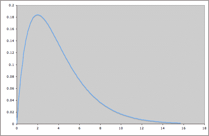
distribution of the random variable. For example, a random
variable might have a probability distribution that looks like this:

The possible values for
the random variable are along the horizontal axis. The height of the
curve above a possible value roughly tells how likely the nearby values
are. This particular
distribution tells us that values of the random variable around 2
(where the curve is highest) are most common, and that very large
values (where the curve is lowest) are uncommon. More precisely, the area under the curve between two
values a and b is the probability that the random variable will take on
values between a and b. In this example, we can see that the
value of the random variable is much more likely to lie between 2 and 4
(where the curve is high) than between 12 and 14 (where the curve is
low).
Notes:
1. See footnote 1 on the page What Is a
Random Sample?
