Dividing a Continuous Variable into Categories

This is also known by other names such as "discretizing," "chopping data," or "binning".¹ Specific methods sometimes used include "median split" or "extreme third tails".

Whatever it is called, it is usually² a bad idea. Instead, use a technique (such as regression) that can work with the continuous variable.The basic reason is intuitive: You are tossing away information. This can occur in various ways with various consequences. Here are some:

1. When doing hypothesis tests, the loss of information when dividing continuous variables into categories typically translates into losing power. ³

2. The loss of information involved in choosing bins to make a histogram can result in a misleading histogram.

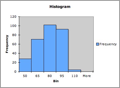
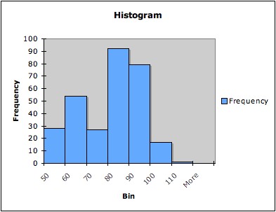
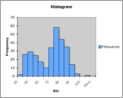
Example: The following three graphs are all histograms of the same data (the times between successive eruptions of the Old Faithful geyser in Yellowstone National Park). The first has five bins, the second seven bins, and the third 14 bins.

Note that that histogram with only five bins does not pick up the bimodality of the data; the histogram with seven bins hints at it; and the histogram with 14 bins shows it more clearly.⁴

3. Collecting continuous data by categories can also cause headaches later on. Good and Hardin⁵ give an example of a long-term study in which incomes were relevant. The data were collected in categories of ten thousand dollars. Because of inflation, purchasing power decreased noticeably from the beginning to the end of the study. The categorization of income made it virtually impossible to correct for inflation.

4. Wainer, Gessaroli, and Verdi⁶ argue that if a large enough sample is drawn from two uncorrelated variables, it is possible to group the variables one way so that the binned means show an increasing trend, and another way so that they show a decreasing trend. They conclude that if the original data are available, one should look at the scatterplot rather than at binned data. Moral: If there is a good justification for binning data in an analysis, it should be "before the fact" -- you could otherwise be accused of manipulating the data to get the results you want!

5. There are times when continuous data must be dichotomized, for example in deciding a cut-off for diagnostic criteria. When this is the case, it is important to choose the cut-off carefully, and to consider the sensitivity, specificity, and positive predictive value. ⁷

Notes:
1. "Binning" is also used to refer to processes used in data mining and analytics. In those fields, which usually deal with large data sets and aim to discover patterns, carefully developed algorithms and validating with holdout subsamples can create a more rigorous process than the types of discretizing discussed on this web page.
2. One situation in which it may be necessary is when comparing new data with existing data where only the categories are know, not the values of the continuous variable. Categorizing may also sometimes be appropriate for explaining an idea to an audience that lacks the sophistication for the full analysis. However, this should only be done when the full analysis has been done and justifies the result that is illustrated by the simpler technique using categorizing. For an example, see Gelman and Park (2008), Splitting a predictor at the upper quarter or third, American Statistician 62, No. 4, pp. 1-8. See also footnote 1 above.
3. See http://psych.colorado.edu/~mcclella/MedianSplit/ for a demo illustrating this in the case when a continuous predictor in regression is dichotomized using a median split. Also see Van Belle (2008) Statistical Rules of Thumb, pp. 139 - 140 for more discussion and references.
4. Some software has a "kernel density" feature that can give an estimate of the distribution of data. This is usually better than a histogram. The problem with bins in a histogram is the reason why histograms are not good for checking model assumptions.
5. Good and Hardin (2006) Common Errors in Statistics, pp. 28 - 29.
6. Wainer, Gessaroli, and Verdi (2006). Finding What Is Not There through the Unfortunate Binning of Results: The Mendel Effect, Chance Magazine, Vol 19, No.1, pp. 49 -52. Essentially the same article appears as Chapter14 in Wainer (2009) Picturing the Uncertain World, Princeton University Press.
7. In addition to the references listed at the end of the linked page, see also Susan Ott's Bone Density page for a graphical discussion of the cut-offs for osteoporosis and osteopenia.