COMMON MISTEAKS
MISTAKES IN
USING STATISTICS: Spotting and Avoiding Them
Misinterpreting the Overall F-Statistic in Regression
Most software includes an "overall F-statistic" and its corresponding
p-value in the output for a least squares regression. This is the
statistic for the hypothesis test with null hypothesis
H0: All non-constant
coefficients in the regression equation are zero
and alternate hypothesis
Ha: At least one of the
non-constant coefficients in the regression equation is non-zero.
More explicitly, if Y is the response variable and the predictors
are X1, X2, ... , Xm and the
model equation1 assumed for the regression is
(*) E(Y|X1, X2,
... , Xm) = β0 + β1 X1+
β2 X2+ ... + βmXm
then the null and alternate hypotheses for this F-test are
H0: β1
= β2 = ... = βm= 0
and
Ha: At least one
of β1,
β2 , ... or βm is non-zero.
Misinterpreting the output for this hypothesis test is a common mistake in regression. Two
types of mistakes are common here.
First type of
mistake: Assuming that if the output for this hypothesis test
has a small p-value, then the regression equation fits the data well.
Second type of
mistake: Assuming that if the output for this hypothesis test
does not show statistical significance, then Y does not depend on the
variables X1, X2, ... , Xm.
Both mistakes are based on neglecting
a model assumption --
namely, the assumption expressed by (*):
that the conditional mean E(Y|X1, X2, ... , Xm)
is a linear function of the
variables X1, X2, ...
, Xm.
Examples of each type of mistake:
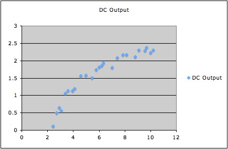
1. The following graph shows DC output vs. wind speed for a windmill.
Running a regression with model assumption
E(DC output|wind speed) = β0
+ β1×(wind speed)
gives overall F-statistic 160.257 with 1 degree of freedom, and
corresponding p-value 7.5455E-12, which is certainly statistically
significant.
However, the data clearly have a curved pattern; thus a model equation
expressing a suitable curved relationship will fit better than a linear
model equation.
(For a good way to do this, see Example 3 of Overinterpreting
High R2.) All that the F-statistic says is that we have
strong evidence that the best
fitting line
has non-zero slope (which is
pretty clear from the picture anyhow).
Of course, in a case with several predictor variables, it is typically
difficult (if not impossible) to tell in advance whether or not a
linear model
fits. Thus, unless there is
other evidence that a linear model does fit, all
that a statistically significant F-test can say is that the data give
evidence that the best-fitting
linear model of the type specified has
at least one predictor with a non-zero coefficient.
One method that sometimes works to get around this problem is to
(attempt to) transform the variables to have a multivariate normal
distribution,
then work with the transformed variables. This will ensure that the
conditional means are a linear function of the transformed explanatory
variables, no matter which subset of explanatory variables is chosen.
Such a transformation is sometimes possible with some variant of a
Box-Cox transformation procedure. See, e.g., pp. 236 and 324 - 329 of
Cook
and Weisberg's text2 for more details.
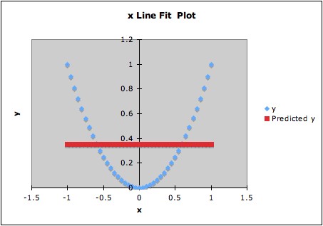
2. The following graph shows data and the computed regression line.
The fitted regression line is y = 0.35 + 0x. The overall F-statistic is
essentially 0, giving p-statistic essentially 1. However, the data are
constructed so that y depends on x: y = x2. Thus there is a
strong dependence of y on x, but the F-test for the linear model does
not detect this at all.
Notes:
1. In the expresion used above, E(Y|X1, X2,
... , Xm) refers to the mean of the conditional
distribution of Y given X1, X2,
... , Xm; see also Overfitting.
Depending on notation used, the model equation might be expressed in
different ways, for example as
Y = β0 + β1
X1+
β2 X2+ ... + βmXm
+ ε
or as
yi = β0 +
β1 xi1+
β2 xi2+ ... + βmxim
+ εi
2. Cook and Weisberg (1999) Applied
Regression Including Computing and
Graphics, Wiley.
Last updated June 13, 2014