ptaylor.py generates an ODE solver in python using the scheme outlined in the previous page. Multi-precision mpfr library and quadmath library (f128) are supported. Jet transport is also supported, although you'll need some basic understanding of jet transport in Taylor to make sense of the output. The generated script outputs the solution to a data file first, then load it back to be used by the other modules in the script (if needed). This IO separation provides a simple mechanism for the script to be used with other python modules. By default, the generated script output the solution to stdout. In the following, we'll explain how to use this script through examples. We'll use the classic Henon-Heiles system for our examples.
usage: ptaylor.py [-h] [-m MODEL_NAME] [-mpfr MPFR] [-f128] [-t0 START_T] [-t1 STOP_T]
[-nsteps NUM_STEPS] [-step STEP_SIZE] [-iv INIT_V] [-sc {0,1,2}] [-abs_err ABS_ERR] [-rel_err REL_ERR]
[-lib SHARED_LIB_NAME] [-o OUTPUT_FILE] [-jlib {1_1,1_n,n_1,2_n,n_2,m_n,tree}] [-d] [-i INPUT_FILE]

optional arguments:
  -h, --help            show this help message and exit
  -m MODEL_NAME, --model_name MODEL_NAME
  -mpfr MPFR, --mpfr_precision MPFR
  -f128, --float128
  -t0 START_T, --start_time START_T
  -t1 STOP_T, --stop_time STOP_T
  -nsteps NUM_STEPS, --num_steps NUM_STEPS
  -step STEP_SIZE, --step_size STEP_SIZE
  -iv INIT_V, --initial_values INIT_V
  -sc {0,1,2}, --stepsize_control {0,1,2}
                        Only 1 is availale when jet var is present
  -abs_err ABS_ERR, --absolute_error_tolerance ABS_ERR
  -rel_err REL_ERR, --relative_error_tolerance REL_ERR
  -lib SHARED_LIB_NAME, --lib_name SHARED_LIB_NAME
  -o OUTPUT_FILE, --output OUTPUT_FILE
  -jlib {1_1,1_n,n_1,2_n,n_2,m_n,tree},
  -i INPUT_FILE, --input INPUT_FILE
Here is the taylor input file for the well known Henon-Heiles system.
x'= xp;
y'= yp;
xp'= -x -2*x*y;
yp'= -y -x^2 + y^2;

expr Hamiltonian= 0.5*(xp^2+yp^2) + 0.5*(x^2+y^2+2*x^2*y -2./3. * y^3);

initialValues=0.0,0.1,0.39,0.2 ;
absoluteErrorTolerance = 1.0E-16;
relativeErrorTolerance = 1.0E-16;
stopTime = 100;
startTime = 0.0;
We added Hamiltonian in the input file. When one or more expressions is tagged along with the ODEs, the generated script will evaluate the expression(s) and output the values following that of the state variables. The time value will be the last number in the output. If there are multiple exressions defined in the input file, only the last definition will be used. We'll check the values of the Hamiltonian along the orbit and see how our solver performs, especially when high precision mpfr arithmetic is used.
The most basic usage is to just use the -i and -o options.
./ptaylor.py -i henon.eq -o ex1.py
If you run ./ex1.py, you'll see an output like the following
  0.00000000000000000 0.10000000000000001 0.39000000000000001 0.20000000000000001 0.10071666666666668 0.00000000000000000
  0.14146921429653089 0.16694583095857063 0.35533127260920483 0.15397458290812380 0.10071666666666666 0.37369311516958242
  0.25350067479984117 0.21056675165705319 0.25502803040927602 0.08339112652402664 0.10071666666666668 0.73465313102724983
  0.31796413315514649 0.22453627186095632 0.10967291266456394 -0.00570822926080773 0.10071666666666666 1.08257375149408386
   ...  ... ...
  0.33469460864047718 0.09257174663790002 0.23280961070109707 0.08019981373364489 0.10071666666666679 98.99711121704999073
  0.38977818353753513 0.10729418698840565 0.07883104920203102 0.00126468133535755 0.10071666666666679 99.34560046563892399
  0.38803476554498956 0.09234490514330268 -0.08793841714914910 -0.08554336650105819 0.10071666666666680 99.69710185083758347
  0.34132800915608263 0.05650298494628910 -0.21640973974319591 -0.14784208527307291 0.10071666666666680 100.00000000000000000
The values of each row are: x, y, xp, yp, Hamiltonian and time. As expected, we see the Hamiltonian is preserved along the orbit, with an error close to 1E-16, the machine ε .
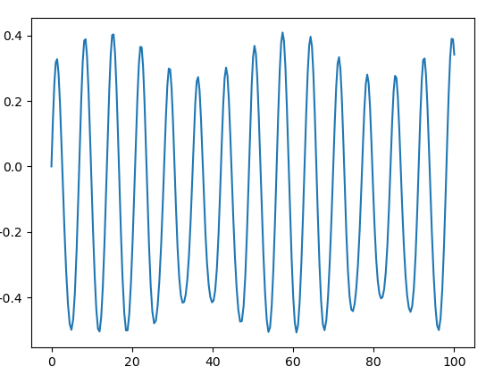
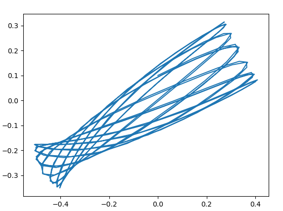
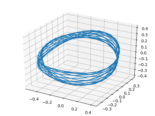
We can also plot the various components of the data with the -p columns option. For example, ./ex1.py -p 6,1 will plot x against time, ./ex1.py -p 1,2 will plot x aganist y and ./ex1.py -p 1,2,3 will produce a 3d plot of x,y and xp.
The generated script support a few command line options. For example, you can change the initial values, the starting and end time etc.
  usage: ex1.py [-h] [-o OUTPUT_FILE] [-p COLUMNS] [-s {dot,solid}] [-t0 START_T] [-t1 STOP_T] [-nsteps NUM_STEPS]
              [-step INITIAL_STEP] [-iv INIT_V] [-sc {0,1,2}] [-abs_err ABS_ERR] [-rel_err REL_ERR] [-d]

  optional arguments:
     -h, --help            show this help message and exit
     -o OUTPUT_FILE, --output_file OUTPUT_FILE
     -p COLUMNS, --plot COLUMNS
                       select columns to plot
     -s {dot,solid}, --style {dot,solid}
                       set plot style
     -t0 START_T, --start_time START_T
     -t1 STOP_T, --stop_time STOP_T
     -nsteps NUM_STEPS, --num_steps NUM_STEPS
     -step INITIAL_STEP, --initial_step INITIAL_STEP
     -iv INIT_V, --initial_values INIT_V
     -sc {0,1,2}, --stepsize_control {0,1,2}
                   Only 1 is availale when jet var is present
     -abs_err ABS_ERR, --absolute_error_tolerance ABS_ERR
     -rel_err REL_ERR, --relative_error_tolerance REL_ERR
     -d, --data            return data in an array [data_array, count]
Let's do one high precision compution. We'll use taylor with the mpfr library. Just for fun, we will use a very high 512 bit precison, about 153 decimal digits. We use the command option to change the default error tolerance from 1E-16 to 1E-150.
./ptaylor.py -mpfr 512 -abs_err 1E-150 -rel_err 1E-150 -i henon.eq -o ex2.py -m ex2
Please note the -m ex2 option. By default, ptaylor.py uses names deduced from the input file for its temp files. For our example, it will by default generate the following temp files tp_ode_name_henon_eq.h, tp_ode_name_henon_eq_step.c and tp_ode_name_henon_eq.c. The compiled shared library will be lib_ode_name_henon_eq.so. The -m ex2 overrides those default names. It provides a method to avoid name clashes when the same input file is used in multiple scripts. In this example, the new temp files are: tp_ex2.h, tp_ex2_step.c and tp_ex2.c. The shared library name will be lib_ex2.so.
If we run ./ex2.py, we'll see a list of numbers each with about 153 digits. In particular, the variations in Hamiltonian are only on the last two digits, close to the ε for our choice of precision.
0.100716666666666674582556832244032962589722161987900303941702774274486085767382608671047985812496007221851735145333500578162325607885681696037257400651773
The sample_main function in ex2.py will return a Python array [data, count] when called with an nonzero argument.
Here, count is the number of data points in data, and data is a column majored matrix whose
columns contain values of x,y,xp,yp etc. Let's use it in a custom program. Let's take
the output data and compute the Hamiltoninan for each point
in the output in our python program. Save the following in henon2.py.
#!/usr/bin/python3
import mpmath
import ex2

def main():
   res,count = ex2.sample_main(1)
   emax= mpmath.mpf(-123456789)
   emin= mpmath.mpf(123456789)
   for i in range(count):
       a=mpmath.fadd(mpmath.fmul(res[2][i], res[2][i]),mpmath.fmul(res[3][i], res[3][i])); # xp^2+yp^2
       b=mpmath.fmul(res[0][i], res[0][i])                             # x^2
       c=mpmath.fmul(res[1][i], res[1][i])                             # y^2
       d=mpmath.fadd(b,c)                                              # x^2+y^2
       e=mpmath.fadd(d, mpmath.fmul(2.0,mpmath.fmul(b, res[1][i])))    # x^2+y^2 + 2 x^2 y
       f=mpmath.fdiv(mpmath.fmul(2.0,mpmath.fmul(c, res[1][i])), 3.0)  # 2./3. * y^3
       g=mpmath.fsub(e,f)                                              # x^2+y^2 +x^2 y - 2/3 y^3
       h=mpmath.fmul(0.5,mpmath.fadd(a, g)) # 0.5*(xp^2+yp^2) + 0.5*(x^2+y^2+2*x^2*y -2./3. * y^3)
       if(h > emax):
          emax = h
       if(h < emin):
          emin = h
   print("EnergyMax",emax)
   print("EnergyMin", emin)
   print("EnergyRange:", mpmath.fsub(emax,emin))

if __name__ == "__main__":
    main()
If you run python3 henon.py -mp , you'll see an output similar to the following.
  EnergyMax 0.100716666666666674582556832244032962589722161987900303941702774274486085767382608671047985812496007221851735145333500578162325607885681696037257400651773
  EnergyMin 0.100716666666666674582556832244032962589722161987900303941702774274486085767382608671047985812496007221851735145333500578162325607885681696037257400651772
  EnergyRange: 1.54760570172404289923287530295855877125561784342958443056134005414030276490204954827425628975808876919751365767558599105158314107975925030205087920214036e-153
It shows the hamiltonian is preserved on the orbit with accuracy of 152 digits. However, if you run the same script without the
-mp option, i.e, invoked as python3 henon.py
you'll get the following output.
  EnergyMax 0.100716666666667
  EnergyMin 0.100716666666667
  EnergyRange: 5.55111512312578e-17
This is because the generated script can load the output data as normal double precision numbers, or as mpmath numbers when mpfr is used. The -mp option tells ex2.sample_main to
load the data using mpmath objects.
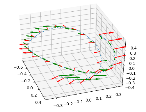
In this example, we demonstrate the jet transport feature in taylor. To that end, we need to modify our input file to add definitions of jet variables and initial values. Save the following in henon3.eq. It declares all our state variables are jet variables of degree 1, with 2 symbols. We essentially tag the first order variational equations w.r.t x and y along with our ODEs.
x'= xp;
y'= yp;
xp'= -x -2*x*y;
yp'= -y -x^2 + y^2;

initialValues=-0.865852,-0.4999,0.0001723368794,0.00009949874371;
absoluteErrorTolerance = 1.0E-16;
relativeErrorTolerance = 1.0E-16;
stopTime = 14;
startTime = 0.0;

jet all symbols 2 degree 1;

jetInitialValues x ="(-0.86659   1 0  )";
jetInitialValues y ="(-0.49990   0 1  )";
jetInitialValues xp ="(0.00017   0 0  )";
jetInitialValues yp ="(0.00099   0 0  )";
Let's generate our script first.
./ptaylor.py -i henon3.eq -o ex3.py -m ex3
When run, each row of the output consists of the values of
x, y, xp, yp, x, u1, v1, y, u2, v2, xp, u3, v3, yp, u4, v4, time
where ui and vi are components of the jet of the corresponding variables.
Let's plot the jets. Save the following in henon3.py
#!/usr/bin/python3
import ex3
import matplotlib.pyplot as plt
from mpl_toolkits.mplot3d import Axes3D
import numpy as np

def main():
    res,count = ex3.sample_main(1)
    fig = plt.figure()
    ax = fig.add_subplot(111, projection='3d')
    plt.plot(res[0],res[1],res[2],linestyle=":")
    zeros=np.zeros(count);
    # x y xp yp x u1 v1 y u2 v2 xp u3 v3 yp u4 v4 t
    u = np.array([res[5],res[6],zeros])
    v = np.array([res[8],res[9],zeros])
    ulength=np.linalg.norm(u)
    vlength=np.linalg.norm(v)
    log_ulength = np.log(ulength)
    log_vlength = np.log(vlength)
    ax.quiver(res[0],res[1],res[2], res[5],res[6],zeros,
    pivot='tail',length=0.4*log_ulength/ulength,arrow_length_ratio=0.3,color="green")
    ax.quiver(res[0],res[1],res[2], res[8],res[9],zeros,
    pivot='tail',length=0.4*log_vlength/vlength,arrow_length_ratio=0.3,color="red")

    plt.show()
if __name__ == "__main__":
   main()
and run it python3 ./henon3.py, you'll see an output similar the following image. The directions of the vectors
are accurate; the lengths are scaled to
0.4 * log(length)/length, the size of the vectors would be too large for the plot without this scaling.