M 408C      Approximating the Change in Rocket Altitude with Riemann Sums  S*(P)           Spring 2002                   

Recall the Rocket Altitude function used in Example 1 of Part IV of the Trapezoid Problem Handout:

Example 1:    Suppose that the function  y  =  f(t)  =  5t²  ,  0  < or =  t  < or = 10,  calculates the altitude (# of feet above

the ground)  of a particular rocket at any time t seconds during the first 10 seconds after its liftoff.

      It is shown there that the formula for the Instantaneous Velocity  (equal to the Instantaneous Rate of Change of the Altitude) at any time  t  is  Velocity = 10 t ft/sec,  which is the same as the formula for the derivative  f '(t)  =  10t ft/sec .

The process of evaluating the derivative   f '(t)   =   allows us to analyze the function which calculates the position of the rocket (here, the altitude) and, through differentiation, determine the rate at which that position is changing (i.e., the velocity) at a particular time.

The process of evaluating an integral allows us to reverse this analysis in some sense; integration allows us to analyze the function which calculates the velocity (i.e., the rate at which the position is changing) and, by calculating the DEFINITE INTEGRAL over an interval of time [a,b] , determine the amount of increase in rocket altitude (i.e., the actual change in position of the rocket) during the interval of time [a,b] .

To motivate the definition of the Integration Process and the definition of the new concepts and new notations  (Partition P of interval [a,b] into  n  sub-intervals, the i^th  sub-interval  ,  width of the i^th sub-interval, etc.), let us consider how the determination of the change in altitude of the rocket from an analysis of the velocity function,  y  =  velocity  =  f(x), might be accomplished.

Suppose that the engineers designing this rocket altered the fuel formula and engine operation so that now its height function and velocity function have changed.  Now the engineers are able to determine that the function, y = f(x) as defined below, calculates the velocity (ft/sec) of the rocket at any time  x seconds during the first  12  seconds after lift-off.  Note that this particular velocity function  f(x) is not in any way an improvement over the one before, but it is designed to be useful for illustrating the integration process.  Also, the variable used for time is  x  now and not  t .

         Here is the new velocity function  y = f(x)  ft/sec velocity at any time  x  ,  0  < or =  x   < or =  12 :

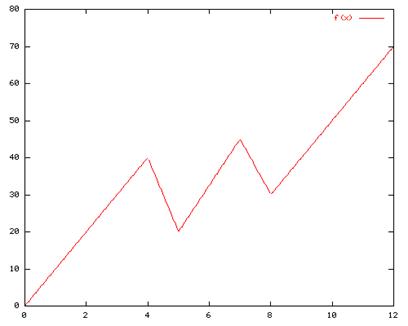
f(x) =

This function does look intimidating, but in fact it will be easy to work with once a few special points on the graph are identified.   Below, the graph is shown again with these special points identified.

A first, very gross, estimate of the increase in altitude during the first 12 seconds of ascent can be found by answering the following question:

Question:  If the rocket velocity had been constant during the whole 12-second interval  [0,12] and if that assumed constant velocity were equal to the actual velocity of the rocket at the end of the interval [0,12], then by how much would the altitude have increased during the whole interval [0,12] ? 

  The velocity at time  x = 12 sec is y = f(12) = 70 feet/sec .  If the rocket traveled at the rate of 70 ft/sec during the complete 12-second interval, then the increase in altitude equals the distance traveled which equals  (rate) (time)  =  (70 ft/sec) (12 sec)  =  840 feet.

Question:  Is this an under-estimation or an over-estimation of the increase in altitude during the interval [0,12] ?              (Answer:    ----------Don't look yet, think about it   ----------------------------  Over-estimation. )

We are going to systematically improve on this approximation by dividing the interval [a,b] = [0,12] into a collection of sub-intervals, that is by forming partitions of the interval [a,b] = [0,12] , and then we will ask what the increase in altitude would have been if the velocity had been constant during each of the sub-intervals of time in the partition of the whole interval of time  [a,b]  =  [0,12]. 

Notation: 

A Partition  P  of an interval [a,b]  is a decomposition of  [a,b]  into a collection of sub-intervals which meet only at endpoints and which join together to fill out the whole interval  [a,b] .  For example,  one partition P of the interval [0,12]  is the collection of  5 sub-intervals:  [0, 4],  [4, 5],  [5, 8],  [8, 11], [11, 12]  .  A Partition P is  specified by listing the endpoints of the sub-intervals in the partition.  Thus, this 5-sub-interval partition is specified by saying, "Partition  P  is the partition  P  =  { 0, 4, 5, 8, 11, 12 }". (A listing of 6 numbers!)

The generic partition P of the generic interval [a,b] is specified as: "P  =  {} , where    and    and  n  is the number of sub-intervals in partition P."

When the interval [a,b] is divided into sub-intervals, the symbol "n" will always represent the number of sub-intervals that the whole interval [a,b] is divided (partitioned) into.

                                                                         REFINEMENT  #1:

We will first partition the 12-second time interval [0,12] into  n = 2  sub-intervals, both of which will conveniently have a width of 6 seconds.    The two sub-intervals are:  [0,6]  and  [6,12] .

Question:  What is the maximum velocity  M₁ of the rocket during the first sub-interval, sub-interval₁ = [0,6] ?

   Answer:     Maximum f(x) velocity value on   =  [0,6]  is   M₁  =   40 ft/sec .  (Refer to graph above)            

Question:  What is the maximum velocity  M₂ of the rocket during the 2^nd  sub-interval, sub-interval₂ = [6,12] ?

   Answer:      Maximum f(x) velocity value on   =  [6,12]  is   M₂  =   70 ft/sec .  (Refer to graph above)            

We are considering here the partition P₁ of  [0,12] , where  P₁  =  { }  =  { 0 , 6, 12 }  which divides the interval [0,12]  into  n = 2  sub-intervals:   =  [0,6]  and    =  [6,12] .   Note:  always represents the last sub-interval in the partition of [a,b] under discussion.

Question:   If the rocket velocity had been constant during each of the two sub-intervals _{, ( i = 1,  2 )} , and if that assumed constant velocity were equal to the maximum actual velocity of the rocket M_i during each sub-interval_i, _{( i = 1,  2 )} ,  then by how much would the altitude have increased during the whole interval [0,12] ?

Answer:    M₁  =   40 ft/sec  is the maximum f(x) velocity on   =  [0,6]  =  sub-interval₁.

                  M₂  =   70 ft/sec  is the maximum f(x) velocity on   =  [6,12]  =  sub-interval₂  = .

  The widths of the sub-intervals (here, lengths of time)  are   =  6 sec  and    =  6 sec.

Thus, with this assumption of constant velocity during each of the sub-intervals, where the constant velocity is the maximum velocity during each sub-interval, the increase in altitude would have been:

         M₁  +   M₂   =   ( 40 ft/sec )  ( 6 sec )  +  ( 70 ft/sec ) ( 6 sec )    =   240  +  420  feet   =   660 feet .

  It is more traditional to write the width of the i^th sub-interval  as   rather that  , and from this point on  will be used to represent the width of the  i^th sub-interval .

Question:  Is this an under-estimation or an over-estimation of the increase in altitude during the interval [0,12] ?              (Answer:    ----------Don 't look yet, think about it.)

          It is an over-estimation because the assumed constant velocity was the maximum of all the velocities attained during each sub-interval, so the actual increase in altitude during each sub-interval was less than the increase in altitude resulting from the assumed constant velocity.

                                                                         REFINEMENT  #2:

We form the partition  P₂  =
  { }  =  { 0 , 3, 6, 9, 12 }  which partitions the interval [0,12] into  n = 4  sub-intervals.    See the graph to the below:

Question:  For each i, i = 1, 2, 3, 4, what is the maximum f(x) velocity M_i  during sub-interval_i ?  That is, what are  M_{i,  ( i = 1,  2, 3, 4 )}  ?    Said another way,  what are  M₁, M₂, M₃,  and   M₄ ?

    M₁ is the maximum f(x) velocity during sub-interval₁  =  [0,3] :  M₁  =  30 ft/sec .  Similarly,  M₂  =  40 ft/sec;  M₃  =  45 ft/sec;   M₄  =  70 ft/sec . 

Question:  What are the widths   , _{( i = 1,  2, 3, 4 )} ,  of the n=4 sub-intervals  ?

  =    =  3 – 0   =   3  sec ,         =    =  6 – 3   =   3  sec .     

  =    =  9 – 6   =   3  sec ,         =    =  12 – 9   =   3  sec .

(Note: The fact that these widths are all the same is a result of our choice at the start to divide the original interval [a,b] = [0,12]  into 4 sub-intervals, all of uniform width.  This "uniform width" choice is NOT REQUIRED and so the 's  are not always constant widths as they are here!)

Question:  What would the increase in altitude have been if the rocket velocity over each sub-interval had been constant and that constant velocity had been the maximum M_i over each sub-interval ?

Answer:   M₁   +   M₂   +   M₃   +   M₄   =    =   (30) (3) + (40) (3) + (45) (3) + (70) (3)  =   90  +  120  +  135  +  210   =  555 feet .     (This is also an over-estimation.)

Definition:  Given function   f ,  given interval [a,b] ,  and  given partition  P  =  { }  with  n  sub-intervals of width , , . . . , ,  and  if, for each  i,  ( i = 1, 2, . . ., n ), M_i = the  Maximum f(x) value on the i^th  sub-interval,   then the   P  Upper  Sum  for  f  ,  U_f  (P) ,  is the summation number:

                                                      U_f  (P)   =   .

Using this terminology, with  the rocket velocity function y = f(x)  for the function f in the definition, and with interval [a,b] = [0,12],  and  with partition  P  =  { 0, 3, 6, 9, 12 } as directly above, then the increase-in-altitude estimate,   M₁   +   M₂   +   M₃   +   M₄   =  555 feet,  shows that the  P  Upper Sum for  f  is:

                                                      U_f  (P)  =    =   555 , where  n = 4 .

                                                        UNDER-ESTIMATE  # 1

Next, we will use the same partition  P₂  =  { 0, 3, 6, 9, 12 }  as before, and we will assume again that  the rocket velocity was constant during each of the sub-intervals, but this time we will assume that the constant velocity during each sub-interval is   m_i  =  the minimum f(x) velocity of all the actual velocities of the rocket attained during the sub-interval.  Thus, looking at the graph above, we see that:

   m₁  =  0 ft/sec  ,  m₂  =  20 ft/sec  ,  m₃  =  30 ft/sec  ,  and  m₄  =  40 ft/sec.   We still have   =  3, _{( i = 1,  2, 3, 4 )} .

With these "minimum f(x) velocity" assumptions, the increase in altitude would have been:

  m₁   +   m₂   +   m₃   +   m₄   =    =   (0) (3) + (20) (3) + (30) (3) + (40) (3)   =  0  +  60  +  90  +  120   =   270  feet .     (This is an under-estimation because minimum f(x) velocities were used for the constant velocities.)

Definition:  Given function   f ,  given interval [a,b] ,  and  given partition  P  =  { }  with  n  sub-intervals of width , , . . . , ,  and  if, for each  i,  ( i = 1, 2, ... , n ),  m_i  =  the  minimum f(x) value on the i^th  sub-interval,   then the   P  Lower  Sum  for  f  ,  L_f  (P) ,  is the summation number:

                                                      L_f  (P)   =   .

Using this terminology, with  the rocket velocity function y = f(x)  for the function f in the definition, and with interval [a,b] = [0,12],  and  with partition  P  =  { 0, 3, 6, 9, 12 } as directly above, then the increase-in-altitude estimate,   m₁   +   m₂   +   m₃   +   m₄   =  270 feet,  shows that the  P  Lower Sum for  f  is:

                                                      L_f  (P)  =    =   270 , where  n = 4 .

Note:  It will always be the case that, no matter what particular partition P  of [a,b] is used, the

                           P  Lower Sum for  f   =  L_f  (P)    < or =      U_f  (P)  =  P  Upper  Sum  for  f   .  ( Why? )

Consider partition  P₃ of [a,b] = [0,12] where   P₃  = { 0, 1, 3, 5, 6, 7.2, 9, 12 }  (here, n = 7) .  The sub-intervals for P₃ are: [0,1] ,  [1,3]  ,  [3,5]  ,  [5,6]  ,   [6, 7.2]  ,  [7.2, 9]  , [9,12]  .    Note how the sub-intervals in P₃ can be collected together into groupings which themselves are partitionings of the sub-intervals in the partition  P₂.

For example,  [0,1] and [1,3]  in  P₃ together make a partition of the sub-interval [1,3]  in  P₂.  Also,  [6, 7.2] and [7.2, 9]  in  P₃ together make a partition of the sub-interval [6,9]  in  P₂.    When this occurs, that is, when the sub-intervals of one partition  P' of [a,b]  form partitionings of the sub-intervals of another partition  P  of [a,b], we say that the partition  P' is  a  Refinement  of the other partition P of [a,b].  

Comparing the Upper and Lower sums of  f  for these two partitions, P and its refinement P', we find that as the refinement of partitions get finer and finer, the P' Lower Sums of  f  get larger and larger and the P' Upper Sums decrease, but still all the Uppers sums are greater that or equal to all the Lower sums.  Thus,  when P' is a refinement of P,             L_f  (P)    < or =      L_f  (P')     < or =      U_f  (P')    < or =      U_f  (P)  .

Looking back at partition  P₃  = { 0, 1, 3, 5, 6, 7.2, 9, 12 }  with interval widths,   = 1 ,  = 2 ,  = 2 ,  = 1 ,  = 1.2 ,  = 1.8 ,  = 3 ,  we can illustrate the concept of the Norm of a partition P, written  || P || ; the Norm of Partition P  is the maximum width of all the widths of the sub-intervals of P.  For P₃, the Norm of P₃ is  || P₃ ||  =  3  =  , here.

Definition of the Definite Integral  I   of  function  f  from  a  to  b:   I  =    .

We can form hundreds of partitions  P  of  interval [a,b] , some having hundreds, thousands, or even hundreds-of-thousands of sub-intervals.   As the number   n , the number of sub-intervals, increases and as the Norm  of the partitions approach  arbitrarily close to 0, the Lower sums  L_f  (P)  increase and the Upper sums   U_f  (P)  decrease and they become closer and closer together, but L_f  (P)  never becomes greater than U_f  (P) .   There is, in fact, only one number,  I,  which can fit in-between all the upper and lower sums of  f  for every partition P of [a,b]. 

That is,  there is one unique number,  I , called "The Definite Integral of  function   f  from  a   to   b" , which is such that, for every partition  P  of  [a,b]  that exists, the number  I  is "in-between" the  P Lower sum of  f  and  the P Upper sum of f ;  and so   L_f  (P)     < or =      I    < or =      U_f  (P)  for every partition  P  of [a,b] .  Thus,

   L_f  (P)       < or =           < or =       U_f  (P)   for every partition  P  of  [a,b], and no other number does this.

Integration is the process of determining this definite integral number I, and it will be the key step in determining the exact increase in the altitude of the rocket, call it , during the first 12 seconds after lift-off.  In fact, we can use logical reasoning to conclude that this number   I  = is  the exact number of  feet by which the altitude increased ;  that is,    =   .

    The argument goes like this:  Given any partition  P  of  [a,b] = [0,12] ,  the  P-Upper sum, U_f  (P), is an estimation of the increase in rocket altitude which assumes that, during each sub-interval of the partition P, the velocity of the rocket was constant and equal to maximum velocity of the rocket during that sub-interval.  The assumption of constant velocity at the maximum velocity of each sub-interval means that this Upper sum estimation will be an over-estimation of the actual increase in altitude:      < or =     U_f  (P) .

  Likewise,  the  P-Lower sum, L_f  (P), is an estimation of the increase in rocket altitude which assumes that, during each sub-interval of the partition P, the velocity of the rocket was constant and equal to the minimum velocity of the rocket during that sub-interval.  The assumption of constant velocity at the minimum velocity of each sub-interval means that this Lower sum estimation will be an under-estimation of the actual increase in altitude:  L_f  (P)   < or =      .

Thus, for every partition P  of  [a,b] = [0,12], we have that:  L_f  (P)   < or =         < or =     U_f  (P)  .   There is only one number that can fit "in-between" all the lower and upper sums of  f, and that number is the Definite Integral  I =    .   Since     also fits "in-between" all the lower and upper sums of  f, it must be true then that      =    .   The techniques of Calculus to be discussed later will enable us to determine that, for   f(x)  =  the rocket velocity function  specified above,   =  412.50 .  Thus, we can conclude that the exact amount of increase in rocket altitude during the first 12 seconds after lift-off was  412.50 feet; that is,

  =    =   412 ½ feet     =    (  ( Altitude at  x = 12 )  –  ( Altitude at  x = 0 )  )

In General,  if   y = f(x)  is a function which calculates the rate of change of another function,  y = F(x), at every number  x  in an interval  [a,b],  (that is, F(x) is a function with  F '(x)  =  f(x) ), then the amount   of net change in the value of  F(x) from  x = a  to  x = b  is equal to the Definite Integral of   f(x)  over the interval [a,b] ;  that is,

     =             =        F(b)  –  F(a)     =      .

                     (This fact is one of the "Fundamental Theorems of Integral Calculus".)

Now, this integral   I  =  is sandwiched in-between all the lower sums  and all the upper sums computed over all partitions  P  of interval [a,b] .   In fact, as the number n, the # of sub-intervals, increases from partition to partition, with n approaching Infinity, and as the maximum sub-interval width, ||P||, approaches 0 ,

 the lower sum for each partition increases  closer and closer to the integeral  I  = .  We summarize this fact by writing:   As    Infinity ,   .   Similarly,  as the maximum sub-interval width, ||P||, approaches 0 ,  the upper sum for each partition decreases  closer and closer to the integeral  I  = .  We summarize this fact by writing: As   Infinity,  .

                                                    Riemann Sums  S*(P)

For a given function  f , and a given interval [a,b] ,  these lower sums and upper sums of  f  for various partitions  P  of   [a,b]  are themselves special cases of a more general calculation to approximate the increase in rocket altitude  ( or to approximate the net change in  F(x) ), a calculation called a Riemann Sum S*(P).

Suppose, for a given partition  P  of  [a,b],  with  n  sub-intervals, we select  n  numbers,  x*₁ from sub-interval₁, x*₂ from sub-interval₂,  . . . , x*_n from sub-interval_n,  that is, we select one  x*_i from each sub-interval of the partition  P.   We approximate the increase in rocket altitude by assuming that the velocity during each sub-interval_i  is the actual velocity  f(x*_i) of the rocket at the selected point x*_i .  The resulting summation approximation is called the   Riemann Sum S*(P)  for  f relative to the choices of x_i*'s :

                           Riemann Sum   .

Some common choices for the x*_i's are these:

    1)   x*_i  =  the left-hand endpoint of sub-interval _i   =  , _{( i = 1,  2, . . ., n)} :   x*_i   =  x _{( i – 1 )  .}

    2)   x*_i  =  the right-hand endpoint of sub-interval _i   =  , _{( i = 1, 2, . . . ,  n )  :}     x*_i   =  x _{i   .}

    3)   x*_i  =  the midpoint of sub-interval _{i , ( i = 1, 2, . . ., n) :}     x*_i   =   .

There are many other possible choices for the x*_i's, and each new selection of the x*_i's can produce a new Riemann Sum  S*(P) calculation.  But, as the partitions  P that we use become finer and finer, as the maximum sub-interval width  ||P||  approaches  0 ,  these Riemann Sum  S*(P) calculations also approach closer and closer to the limit  I  =    .   We summarize this fact by writing:

                 As   Infinity ,  .   That is,  as  Infinity, .

It is this fact, in fact, that explains why the notation for the definite integral is what it is:  the notation reminds us that this special number,  I  =    is  the limit of  sums of terms, each of which is a product of the form   computed over the interval  [a,b] .  We can imagine that, in the limit process, the turn into the symbol,  the  f(x*_i)'s turn into the function  f(x), and the 's  turn into  dx .

In the rest of this handout, we will use geometry to verify that the number  I  =   is actually equal to  412.5, and so for the rocket velocity function f(x) we have been analyzing, the increase in rocket altitude in the first 12 seconds after lift-off is actually 412.5 feet.

   But first, it is important to mention one important fact about the possible values of the definite integral

I  =   .  That is,  if the function  f(x)  is continuous and is such that  y = f(x)  <  0  for every  , then the definite integral   I  =   is also  negative,  that is,     <  0  also.  This is because, for every partition P of [a,b],  the maximum f(x)-values  M_i on the sub-intervals will themselves be negative numbers and the upper sums,   U_f  (P)  =  , will all be negative totals also.  These upper sums will decrease (become even more negative) down toward the definite integral  ,  which must then be negative too.  It is even possible that, on one sub-interval of [a,b],  y = f(x) < 0,  and on another sub-interval of [a,b], y = f(x) > 0, in such a way that  I  =   =  0  .

                   Geometrical Verification that       =    =   412 ½ feet

We have seen that    =    already, but we can use geometry to show that    =  412.5.

OBSERVATION:  When   y = f(x) > or = 0  on  [a,b],  and when  P  is a partition of interval [a,b], and when numbers 's  have been chosen from the sub-interval_i's,  then  for each  term   ,  calculated when computing the summation  S*(P) ,  that term also calculates the area of a rectangle on the graph of  y = f(x); it is the area of the rectangle built with base along the x-axis, situated directly on sub-interval_i, and with the height of the rectangle equal to the function value f(x_i) at the selected point x_i in that i^th  sub-interval.

The Rieman Sum S*(P) is the summation of these terms, and this summation is also the summation of the areas of these rectangles, and so the summation  S*(P) can be viewed as an approximation to the area  A_Curve of the region of the plane which lies under the curve  y = f(x), above the x-axis, and between the lines x = a  and x = b , two lines which are perpendicular to the x-axis at the endpoints of the given interval [a,b].

For example, we compute the Riemann Sum S*(P) using the  rocket velocity function  y = f(x)  defined at the start of this handout, and using the partition  P₂  =  { 0, 3, 6, 9, 12 } ,  and using a particular selection of  numbers for the x*_i's, namely,   x*₁ = 1.5,   x*₂  =  4.5,   x*₃  =  7.5  and  x*₄ = 11 .  The relevant function values are f(x*₁)  =  f(1.5)  =  15 ;  f(x*₂)  =  f(4.5)  =  30 ;  f(x*₃)  =  f(7.5)  =  37.5 ;   and  f(x*₄)  =  f(11)  =  60 .  The sub-interval widths are all    = 3 .  Thus, the Riemann Sum S*(P) here is:

 S*(P)   =  =  (15) (3)  +  (30) (3)  +  (37.5) (3)  +  (60) (3)    =   427.5 .  This is also the sum of the areas of the rectangles shaded in the graph below:

The 1^st  rectangle has area   =  f(1.5) *  = (15)*(3)  =  45 .

The 2^nd  rectangle has area  =  f(4.5) *   = (30)*(3)  =  90 .

The 3^rd  rectangle has area  =  f(7.5) *   =  (37.5)*(3)  =  112.5 .

The 4^th  rectangle has area  =  f(11) *  = (60)*(3)   =  180.

The total area of the shaded region is               45 + 90 + 112.5 + 180  =  427.5  =  S*(P) .

S*(P)  =  the area of this shaded region !

Now, since all of the Riemann Sums S*(P) for this function f(x) and  for all the partitions of [a,b] can be viewed as calculating the sum of areas of rectangles and as approximations of  A_Curve ,  the area under the curve and above the interval [a,b] on the x-axis, so too can all the Upper sums U_f (P)  and all of the Lower sums  L_f (P) be viewed as approximations to this area.  But, when we compare these L_f (P)  and U_f (P) approximations to the actual area under curve,  A_Curve , we find that, for all partitions  P,

                                                       L_f  (P)   < or =    A_Curve    < or =   U_f  (P)   .

  For example, the graphs below demonsrate this using the partition  P  =  P₂ :

  For the computation of   L_f  (P) , in the summation  S*(P),  we will use the following as the selected numbers:  For the i^th sub-interval, = that number  x in the sub-interval such that  f()  =  m _i .   In this case then,

L_f (P)  =  S*(P)  =

           =  (0)(3) + (20)(3) + (30)(3) + (40)(3)

           =    0  +  60  +  90  +  120   =   270 

           = the area of the shaded region.

For the computation of   U_f  (P) , in the summation  S*(P),  we will use the following as the selected numbers :  For the i^th sub-interval, = that number x in the sub-interval such that  f()  =  M _i .   In this case then,

U_f (P)  =  S*(P)  =

        =  (30)(3) + (40)(3) + (45)(3) + (70)(3)

        =  90  +  120  +  135  +  210   =   555   

        =  the area of the shaded region.

If you look closely at the two graphs above, you will see that the region with the area equal to L_f (P) lies completely within the region under the curve.  If you think about it, you will see that this is going to be true for every partition  P of  [a,b] = [0,12] .  So, for every partition  P of  [a,b],    L_f (P)  < or =  A_Curve  =  the area under the curve.

You will also see that the region under the curve lies completely within the region with the area equal to U _f (P), and this will be true for all partitions P of [a,b]  =  [0,12] .  So, for every partition  P of  [a,b],   A_Curve   < or =   U_f (P) .

Since the area under the curve   A_Curve  is "in-between" all of the Lower sums and all of the Upper sums of all partitions  P  of  [a,b]  =  [0,12] , it must also be true that A_Curve  is equal to that special number  I  =  .

The region under this particular curve is made up of a triangle and  four (4) trapezoids,  formed by drawing vertical lines perpendicular to the x-axis at  x =  4, 5, 7, and 8.   It is a simple matter to calculate the areas of these trapezoids, and the sum their areas is  equal to  412.5 square units.  This verifies the earlier assertion that   =   412.5  and verifies that the increase in rocket altitude during the first 12 seconds after lift-off  is exactly 412.5  feet.