Frequentist Hypothesis Tests, p-values, and Type I Error

COMMON MISTEAKS MISTAKES IN USING STATISTICS: Spotting and Avoiding Them

Introduction Types of Mistakes Suggestions Resources Table of Contents About Glossary Blog

Frequentist Hypothesis Tests and p-values

As discussed on the page Overview of Frequentist Hypothesis Tests, most commonly-used frequentist hypothesis tests involve the following elements:

   1. Model assumptions
   2. Null and alternative hypothesis
   3. A test statistic. This needs to have the property that extreme values of the test statistic cast doubt on the null hypothesis.
   4. A mathematical theorem saying, "If the model assumptions and the null hypothesis are both true, then the sampling distribution of the test statistic has this particular form."

The exact details of these four elements will depend on the particular hypothesis test; see the page linked above for elaboration in the case of the large sample z-test for a single mean.

The discussion on that page does not go into much detail on the concept of sampling distribution. This page will elaborate on that. First, read the page Overview of Frequentist Confidence Intervals, which illustrates the idea of sampling distribution for the sample mean. Then read the following adaptation of that idea to the situation of a one-sided t-test for a population mean. This will illustrate the general concepts of of p-value and hypothesis testing as well as sampling distribution for a hypothesis test.

We are considering a random variable Y which is normally distributed. (This is one of the model assumptions.)
Our null hypothesis is: The population mean µ of the random variable Y is a certain value µ₀.
For simplicity, we will discuss a one-sided alternative hypothesis: The population mean µ of the random variable Y is greater than µ₀. (i.e., µ> µ₀)
Another model assumption says that samples are simple random samples. We have data in the form of a simple random sample of size n.
To understand the idea behind the hypothesis test, we need to put our sample of data on hold for a while and consider all possible simple random samples of the same size n from the random variable Y.

For any such sample, we could calculate its sample mean ȳ and its sample standard deviation s.
We could then use ȳ and s to calculate the t-statistic t = (ȳ - µ₀)/(s/√n)
Doing this for all possible simple random samples of size n from Y gives us a new random variable, T_n. Its distribution is called a sampling distribution.
The mathematical theorem associated with this inference procedure (one-sided t-test for population mean) tells us that if the null hypothesis is true, then the sampling distribution has what is called the t-distribution with n degrees of freedom. (For large values of n, the t-distribution looks very much like the standard normal distribution; but as n gets smaller, the peak gets slightly smaller and the tails go further out.)

Now consider where the t-statistic for the data at hand lies on the sampling distribution. Two possible values are shown in red and green, respectively, in the diagram below. Remember that this picture depends on the validity of the model assumptions and on the assumption that the null hypothesis is true.

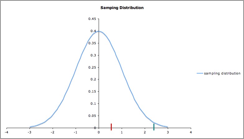
If the t-statistic lies at the red bar (around 0.5) in the picture, nothing is surprising; our data are consistent with the null hypothesis. But if the t-statistic lies at the green bar (around 2.5), then the data would be fairly unusual -- assuming the null hypothesis is true. So a t-statistic at the green bar would cast some reasonable doubt on the null hypothesis. A t-statistic even further to the right would cast even more doubt on the null hypothesis.¹

p-values

We can quantify the idea of how unusual a test statistic is by the p-value. The general definition is:

p-value = the probability of obtaining a test statistic at least as extreme as the one from the data at hand, assuming the model assumptions and the null hypothesis are all true.

Recall that we are only considering samples, from the same random variable, that fit the model assumptions and of the same size as the one we have. ²

So the definition of p-value, if we spell everything out, reads

p-value = the probability of obtaining a test statistic at least as extreme as the one from the data at hand, assuming the model assumptions are all true, and the null hypothesis is true, and the random variable is the same (including the same population), and the sample size is the same.

Comment: The preceding discussion can be summarized as follows:

If we obtain an unusually small p-value, then (at least) one of the following must be true:

At least one of the model assumptions is not true (in which case the test may be inappropriate)
The null hypothesis is false
The sample we have obtained happens to be one of the small percentage that result in a small p-value.

The interpretation of "at least as extreme as" depends on the alternative hypothesis:

For the one-sided alternative hypothesis µ> µ₀ , "at least as extreme as" means "at least as great as". Recalling that the probability of a random variable lying in a certain region is the area under the probability distribution curve over that region, we conclude that for this alternative hypothesis, the p-value is the area under the distribution curve to the right of the test statistic calculated from the data. (Note that, in the picture, the p-value for the t-statistic at the green bar is much less than that for the t-statistic at the red bar.)
Similarly, for the other one-sided alternative µ< µ₀ , the p-value is the area under the distribution curve to the left of the calculated test statistic. (Note that for this alternative hypothesis, the p-value for the t-statistic at the green bar would be much greater than the t-statistic at the red bar, but both would be large as p-values go; in particular, the green value would be even more unusual for this alternate hypothesis than for the null hypothesis.)
For the two-sided alternative µ≠ µ₀, the p-value would be the area under the curve to the right of the absolute value of the calculated t-statistic, plus the area under the curve to the left of the negative of the absolute value of the calculated t-statistic. (Since the sampling distribution in the illustration is symmetric about zero, the two-sided p-value of, say the green value, would be twice the area under the curve to the right of the green bar.)

Note that, for samples of the same size², the smaller the p-value, the stronger the evidence against the null hypothesis, since a smaller p-value indicates a more extreme test statistic. If the p-value is small enough (and assuming all the model assumptions are met), rejecting the null hypothesis in favor of the alternate hypothesis can be considered a rationale decision.

Comments:

How small is "small enough" is a judgment call.
"Rejecting the null hypothesis" does not mean the null hypothesis is false or that the alternate hypothesis is true.

These comments are discussed further on the page Type I and II Errors.

1. A little algebra will show that if t = (ȳ - µ₀)/(s/√n) is unusually large, then so is ȳ, and vice-versa.

2. Comparing p-values for samples of different size is a common mistake. In fact, larger sample sizes are more likely to detect a difference, so are likely to result in smaller p-values than smaller sample sizes, even though the context being examined is exactly the same.

Last updated Jan 20, 2013