COMMON MISTEAKS
MISTAKES IN
USING STATISTICS: Spotting and Avoiding
Them
Power of a Statistical Procedure
"...
power calculations ... in general are more delicate than questions
relating to Type I error."
B.
Efron (2010), Large-Scale
Inference: Empirical Bayes Methods for Estimation, Testing, and
Prediction, Cambridge, p. 85
Overview
The power
of a
statistical procedure can be thought of as the probability
that the
procedure will
detect a true difference of a specified type. As in talking
about
p-values and confidence levels, the
reference category for "probability" is
the sample. So spelling this out in
detail:
Power is the probability that a
randomly chosen sample
satisfying the model assumptions will detect a difference of the
specified type when the procedure is applied, if the specified
difference does indeed occur in the population being studied.
Note also
that power is a conditional probability:
the probability of detecting a difference, if indeed the difference
does exist.
In many real-life situations, there are reasonable conditions that we
would be interested in being able to detect, and others that would not
make a
practical difference.
Examples:
- If you can only measure the response to
within 0.1
units, it doesn't really make sense to worry
about falsely rejecting a null hypothesis for a mean when the actual
value of the mean is within less than 0.1 units of the value specified
in the null hypothesis.
- Some differences are of no practical
importance -- for
example, a medical treatment that extends life by 10 minutes is
probably not worth it.
In cases such as these, neglecting power could result in one or more of
the following:
- Doing much
more
work than necessary
- Obtaining results which are meaningless,
- Obtaining results that don't answer the
question of
interest.
Elaboration
For a
confidence
interval procedure, power can be defined as the probability1
that the procedure will produce an interval with a half-width of at
least a specified amount2.
For a
hypothesis test, power can be defined as the probability1
of rejecting the null hypothesis under a specified condition.
Example:
For a one-sample t-test
for the mean of a population, with null hypothesis H0:
µ = 100,
you might be interested in the probability of rejecting H0
when µ
≥ 105, or when |µ - 100| > 5, etc.
As with Type II error, we need to
think of power in terms of power
against a specific alternative rather
than against a general alternative.
Example:
If we are performing a
hypothesis test
for the mean of a population, with null hypothesis H0:
µ = 0, and
are interested in rejecting Ho when µ > 0, we might
(depending on the situation -- i.e., on what difference is of practical
significance) calculate the power of the test against
the specific alternative H 1:
µ = 1, or against the specific alternate H3
:
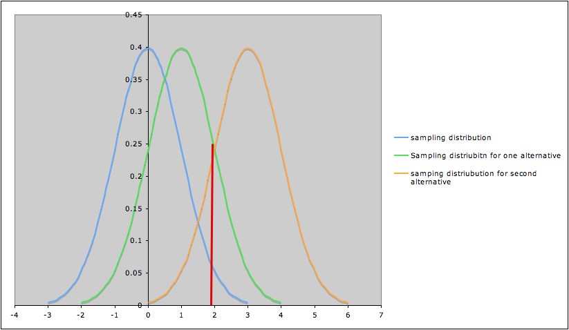
µ = 3, etc. The picture below shows three
sampling distributions:
- The sampling distribution assuming H0
(blue; leftmost curve)
- The sampling distribution assuming H1
(green; middle curve)
- The sampling distribution assuming H3
(yellow; rightmost curve)
The red line marks the cut-off corresponding to a
significance level α = 0.05.
- Thus the area under the blue curve to the right of the red
line is 0.05.
- The area under the green
curve the to right of the red line
is the probability of rejecting the
null hypothesis (µ = 0) if the specific
alternative H1: µ
= 1 is true. In other words, this
area is the power of the test
against the specific alternative H1: µ = 1. We
can see in the picture that in this case,
this power is greater than 0.05, but noticeably less than 0.50.
- Similarly, the area under the yellow curve
the to right of the red line
is the power
of the test against the
specific alternative H3: µ = 3.
Notice that it is much larger than 0.5.
This illustrates the general phenomenon that the farther an alternative is from the
null hypothesis, the higher the power of the test to detect it. 3
Note: For most
tests, it is possible to
calculate the power against a specific
alternative, at least to a reasonable approximation, if relevant
information (or good approximations to them) is available. It is not usually possible to
calculate the power against
a general alternative, since the general alternative is made up of
infinitely many possible specific alternatives.
Power and
Type II Error
Recall that the Type II Error
rate β
of a test against a specific alternate hypothesis test is represented
in the diagram above as the area under the sampling distribution curve
for that alternate hypothesis and to the left
of the cut-off line for the test. Thus
(Power of a test against a
specific alternate hypothesis) + β
= total area under sampling distribution curve = 1,
so
Factors
that Influence Power
In addition to the alternative or other degree of
difference (e.g., width of confidence interval) desirable to detect, sample size, variance, and experimental design influence
power. More
Detrimental Effects of
Underpowered or Overpowered Studies
Common Mistakes Involving
Power
Notes:
1. Again, the reference category
for
the probability is the samples.
2. This assumes a confidence interval procedure that results in a
confidence interval centered at the parameter estimate. Other
characterizations may be needed for other types of confidence interval
procedures.
3. The Rice Virtual Lab in Statistics' Robustness
Simulation can be used to illustrate, in an interactive manner, the
effect of the difference to be detected (and also of standard
deviation), on
power for the two-sample t-test.
Last updated August 28,
2012
