Surfaces and traces

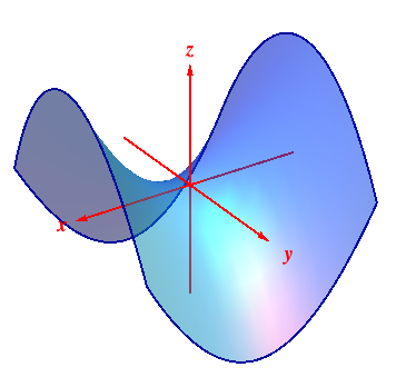
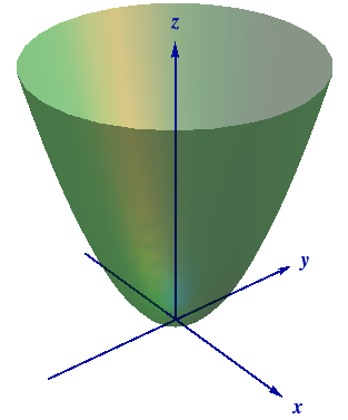
We've already seen surfaces like planes, circular cylinders and spheres. The next step is to look at a surface arising as the graph of a real-valued function $z = f(x,\, y) : U \subseteq {\mathbb R}^2 \to {\mathbb R}$ of two variables - in practice, such functions occur in the theory of heat flow in a bar, or vibrating strings, or the pressure at a point on the earth. The graph of $z = f(x,\, y)$ is the surface $$\color{rgb(0, 51, 153)} {S \ = \ \big\{ (x,\, y, \, f(x,\, y)\big) : \, \ (x,\, y) \ \hbox{in} \ U\, \big\} }$$ in $3$-space. Two examples that will occur repeatedly are shown below in

$$ z \ = \ f(x,\, y) \ = \ x^2 - y^2$$

$$\color{rgb(0, 102, 0)}{ z \ = \ f(x,\, y) \ = \ x^2 + y^2}$$

How do we know the surfaces look like that? The basic idea is to take cross-sections of the surface by plane slices. Because a plane intersects the surface in a curve that also lies in the plane, this curve is often referred to as the trace of the surface on the plane. Identifying traces gives us one way of 'picturing' the surface; re-assembling the cross-sections then provides a full picture of the surface. It thus reduces the problem of describing a surface to identfying curves in the plane - the 'natural progression' idea at work! When $z = f(x,\, y)$,

  the trace on a vertical plane $y=mx+b$ is the curve consisting of all points $$\big\{\, (x,\, mx+b,\, f(x,\, mx+b))\,:\ (x,\, mx+b) \ \hbox{in} \ D\, \big\},$$ in the plane $y = mx + b$,

  the trace on a horizontal plane $z = c$ is the curve $$\big\{\, (x,\, y,\, c) :\, (x,\, y) \ \, \hbox{in}\, \ D,\ f(x,\,y) = c\ \big\}$$ in the plane $z = c$.

In the case $z = x^2 - y^2$ slicing vertically by $y = b$ means fixing $y = b$ and graphing $$z \ = \ f(x,\, b) \ = \ x^2 - b^2\,,$$ while slicing vertically by the plane $x = a$ gives $$z \ = \ f(a,\, y) \ = \ a^2 - y^2\,,$$ i.e., parabolas opening up and down respectively.

On the other hand, slicing horizontally by $z = c$ gives $$\ f(x,\,y) \ = \ c \ = \ x^2 - y^2\,,$$ i.e., hyperbolas opening in the $x$-direction if $c > 0$ and in the $y$-direction if $c < 0$. So the cross-sections are parabolas or hyperbolas, and the surface is called a hyperbolic paraboloid. You can think of it as a saddle or as a Pringle!