Main page
Chapter 10: Parametric Equations and Polar Coordinates
Chapter 12: Vectors and the Geometry of Space
Chapter 13: Vector Functions
Chapter 14: Partial Derivatives
Learning module LM 14.1: Functions of 2 or 3 variables:
Learning module LM 14.3: Partial derivatives:
Learning module LM 14.4: Tangent planes and linear approximations:
Learning module LM 14.5: Differentiability and the chain rule:
Learning module LM 14.6: Gradients and directional derivatives:
GradientsGradients and hill climbing
Wind and weather
Directional derivatives
Worked problems
Learning module LM 14.7: Local maxima and minima:
Learning module LM 14.8: Absolute maxima and Lagrange multipliers:
Chapter 15: Multiple Integrals
Gradients
| Definition: the Gradient of a real-valued function $z = f(x, \,y)$ is the vector function $$(\nabla f)(x, \,y)\ = \ \frac{\partial f}{\partial x}\, {\mathbf i} \, +\, \frac{\partial f}{\partial y}\, {\mathbf j}$$ whose components are the partial derivatives of $f$ in the $x$- and $y$-directions. |
This definition generalizes immediately to a function $w = f(x,\,y,\, z)$: $$(\nabla f)(x,\,y,\, z) \ = \ \frac{\partial f}{\partial x}\, {\mathbf i} + \frac{\partial f}{\partial y}\, {\mathbf j} + \frac{\partial f}{\partial z}\, {\mathbf k}\,.$$
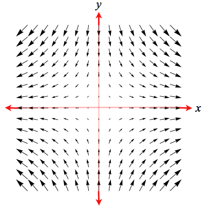
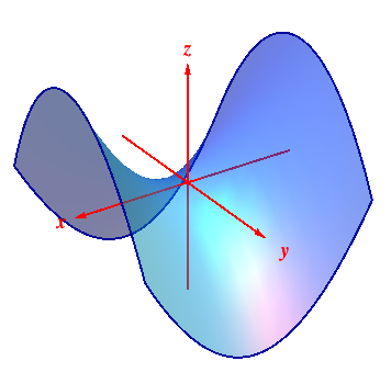
| Example: for $f(x,\,y)= x^2 - y^2$, $$(\nabla f)(x,\, y) \ = \ 2x\,{\mathbf i} -2y\,{\mathbf j}\,.$$ To draw the graph of $\nabla f$ we select a set of points $P(x,\,y)$ and represent $(\nabla f)(P)$ by a vector with initial point $P$ and length scaled so that it's not too long but remains a fixed proportion of the true length of $(\nabla f)(P)$. Drawing $(\nabla f)(P)$ for every $P$ is not helpful, of course, because it would cover the plane with arrows, so we choose a representative set. But for functions of $3$ or more variables, the graph of $\nabla f$ is usually too cluttered to be of much use even if a computer graphics program is used. |
|
|
|

