M408M Learning Module Pages

Main page

Linear regression

Bonus material: Linear regression

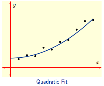
Linear Regression: There are many other applications of optimization. For example, 'fitting' a curve to data is often important for modelling and prediction. To the left below, a linear fit seems appropriate for the given data, while a quadratic fit seems more appropriate for the data to the right.

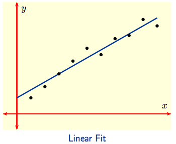
But what does 'best' fit mean and how might we determine that best fit? We'll see how this works for the `best line'. This is an optimization problem which for the linear case can be formulated as minimizing a function of two variables. The `best quadratic fit' uses many of the same ideas, but is a bit more complicated.

Suppose an experiment is conducted at times

$x_1,\, x_2, \, \dots \, x_n$ yielding observed values

$y_1,\, y_2, \, \dots \, y_n$ at these respective times. If the points

$(x_j,\, y_j),\ 1 \le j \le n,$ are then plotted and they look like ones the to left above, one might conclude that the experiment can be described mathematically by a Linear Model indicated by the line drawn through the data. Using

$y = mx + b$ for the equation of the model line, we get predicted values

$p_1,\, p_2, \, \dots \, p_n$ at

$x_1,\, x_2, \, \dots \, x_n$ by setting

$p_j = mx_j + b$ . The difference

$p_j - y_j = mx_j + b - y_j$ between the predicted and observed values is a measure of the error at the

$j^{\hbox{th}}$ -observation: it measures how far above or below the model line the observed value

$y_j$ lies. We want to minimize the total error over all observations.

The minimum value of the sum $E(m,\,b) \ = \ (p_1 - y_1)^2 + (p_2 - y_2)^2 + \ldots + (p_n - y_n)^2\qquad \qquad \qquad \qquad\qquad$ $\qquad \qquad \qquad \ = \ ( mx_1 + b - y_1)^2 + ( mx_2 + b - y_2)^2 + \ldots + ( mx_n + b - y_n)^2$ as $m,\ b$ vary is called the least squares error. For the minimizing values of $m$ and $b$ , the corresponding line $y = mx + b$ is called the least squares line or the regression line.

Taking squares

$(p_j - y_j)^2$ avoids positive and negative errors canceling each other out. Other choices like

$|p_j - y_j|$ could be used, but since we'll want to differentiate to determine

$m$ and

$b$ , the calculus will be a lot simpler if we don't use absolute values!!

In the following video, we derive the equations for a least squares line and work an example.

For your convenience, we repeat the calculation in text form:

To determine the critical point of $E(m,\, b)$ we compute the components of the gradient and set them equal to zero:

$\frac{\partial E}{\partial m} \ = \ 2\left(x_1(m x_1 + b-y_1) + x_2(mx_2 + b- y_2) + \ldots + x_n(mx_n + b - y_n)\right) \ = \ 0\,,$

$\frac{\partial E}{\partial b} \ = \ 2\left((m x_1 + b-y_1) + (mx_2 + b- y_2) + \ldots + (mx_n + b - y_n)\right) \ = \ 0\,,$ After rearranging terms, we get

$\begin{eqnarray*}0 \ = \ \frac{\partial E}{\partial m} &=& 2\Big(\big(x_1^2 + x_2^2 + \ldots + x_n^2\big)m + \big(x_1 + x_2 + \ldots + x_n\big)b -\big(x_1y_1 + x_2y_2 + \ldots + x_n y_n\big)\Big), \cr \cr 0 \ = \ \frac{\partial E}{\partial m} &=& 2\Big(\big(x_1 + x_2 + \ldots + x_n\big)m + \big(1 + 1 + \ldots + 1\big)b -\big(y_1 + y_2 + \ldots + y_n\big)\Big)\,.\end{eqnarray*}$ That's two linear equations in

$m$ and

$b$ , and solving two linear equations in two unknowns isn't hard. In fact, most spreadsheet programs or computer algebra systems have a built-in algorithm for calculating

$m$ and

$b$ to determine the regression line for a given data set. Here's how they do it.

Dividing the two equations by $2$ and rearranging terms gives the system of equations

$\begin{eqnarray*} \left ( \sum_{i=1}^n x_i^2 \right ) m + & \left (\sum_{i=1}^n x_i \right ) b & \ = \ \sum_{i=1}^n x_i y_i, \cr \left ( \sum_{i=1}^n x_i \right ) m + & nb & \ = \ \sum_{i=1}^n y_i. \end{eqnarray*}$ Instead of looking at sums, it's convenient to look at averages, which we denote with angle brackets. Let

$\langle x\rangle \ = \ \frac{1}{n} \sum_{i=1}^n x_i, \qquad \langle x^2 \rangle \ = \ \frac{1}{n}\sum_{i=1}^n x_i^2, \qquad \langle y \rangle \ = \ \frac{1}{n}\sum_{i=1}^n y_i, \qquad \langle xy \rangle \ = \ \frac{1}{n}\sum_{i=1}^n x_i y_i.$ After dividing by

$n$ , our equations become

$\begin{eqnarray*} \langle x^2 \rangle m + & \langle x \rangle b \ = \ & \langle xy \rangle, \cr \langle x \rangle m + & \phantom{\langle x \rangle} b \ = \ & \langle y \rangle. \end{eqnarray*}$ The first equation minus

$\langle x \rangle$ times the second equation gives

$\left ( \langle x^2 \rangle - \langle x \rangle^2 \right ) m \ = \ \langle xy \rangle - \langle x \rangle \langle y \rangle,$ which we can solve for

$m$ . Plugging that back into the second equation gives

$b$ . The results are

The equations of the least squares line through the points $(x_1,y_1)$ , $(x_2,y_2), \ldots, (x_n,y_n)$ is $y=mx+b$ , where $\begin{eqnarray*} m \ = \ & \displaystyle{ \frac{\langle xy \rangle - \langle x \rangle \langle y \rangle} {\langle x^2 \rangle - \langle x \rangle^2}} & \ = \ \frac{\displaystyle{n \left (\sum_{i=1}^n x_iy_i\right ) - \left ( \sum_{i=1}^n x_i\right ) \left ( \sum_{i=1}^n y_i\right )}} {\displaystyle{n\left ( \sum_{i=1}^n x_i^2\right ) - \left (\sum_{i=1}^n x_i \right )^2}}, \cr \cr b \ = \ & \frac{\displaystyle{\langle x^2 \rangle\langle y \rangle - \langle x \rangle \langle xy \rangle}} {\displaystyle{\langle x^2 \rangle - \langle x \rangle^2}} & \ = \ \frac{\displaystyle{\left ( \sum_{i=1}^n x_i^2\right ) \left ( \sum_{i=1}^n y_i \right ) - \left ( \sum_{i=1}^n x_i\right ) \left (\sum_{i=1}^n x_i y_i \right )}} {\displaystyle{n\left (\sum_{i=1}^n x_i^2 \right ) - \left (\sum_{i=1}^n x_i \right )^2}}. \end{eqnarray*}$

Chapter 10: Parametric Equations and Polar Coordinates

Chapter 12: Vectors and the Geometry of Space

Chapter 13: Vector Functions

Chapter 14: Partial Derivatives

Learning module LM 14.1: Functions of 2 or 3 variables:

Learning module LM 14.3: Partial derivatives:

Learning module LM 14.4: Tangent planes and linear approximations:

Learning module LM 14.5: Differentiability and the chain rule:

Learning module LM 14.6: Gradients and directional derivatives:

Learning module LM 14.7: Local maxima and minima:

Learning module LM 14.8: Absolute maxima and Lagrange multipliers:

Chapter 15: Multiple Integrals

Linear regression