Examples

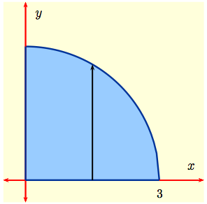
Example 1: Evaluate the integral $$I \ = \ \int \int_D\, (x+y)\, dA$$ when $D$ consists of all points $(x,\,y)$ such that $$0 \ \le \ y \ \le \sqrt{9-x^2}\,, \quad 0\ \le \ x \ \le 3\,.$$ Since $y^2 \ = \ 9 - x^2$ is a circle of radius $3$ centered at the origin, $D$ consists of all points in the first quadrant inside this circle as shown to the right. This is a Type I region, which suggests      Fixing $x$ and integrating with respect to $y$ along the black vertical line as shown, and      Then integrating with respect to $x$. So the double integral $I$ becomes the repeated integral $$\int_0^3\left(\int_0^{\sqrt{9-x^2}}\, (x+y)\, dy\right)dx= \int_0^3\, \Bigl[\, xy + \frac{1}{2}y^2 \,\Bigl]_0^{\sqrt{9 - x^2}}\,dx.$$

Thus $$I\ = \ \int_0^3\, \Bigl( x\sqrt{9 - x^2} + \frac{1}{2} (9 - x^2)\Bigr)\, dx\ = \ 18\,.$$ How would you evaluate this last integral?

In Example 1 algebraic conditions specifying $D$ suggested how to write the integral as a repeated integral. Other times algebraic conditions are best interpreted graphically before deciding on limits of integration.

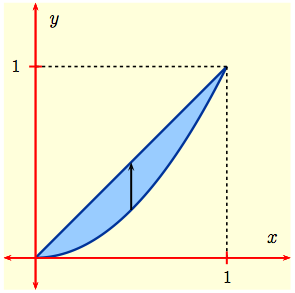
Example 2: Evaluate the integral $$I \ = \ \int \int_D\, (3x +4y)\, dA$$ when $D$ is the bounded region enclosed by $y = x$ and $y=x^2$. Here $D$ is enclosed by the straight line $y = x$ and the parabola $y = x^2$ as shown to the right. To determine the limits of integration we first need to find the points of intersection of $y = x$ and $y = x^2$. These occur when $x^2 = x$, i.e., when $x = 0,\, 1$. Treating $D$ as a Type I region, we fix $x$ and integrate with respect to $y$ along the black vertical line, getting the repeated integral $$ I \ = \ \int_0^1\left(\int_{x^2}^{x}\, (3x + 4y)\, dy\right)dx$$

Can you now evaluate $I$?

In Example 2 it was simpler to fix $x$ and integrate first with respect to $y$ because the bounding curves were already given to us as $$y \ = \ f_1(x)\ = \ x^2\,,\qquad y \ = \ f_2(x)\ = \ x\,.$$ Had they been given as $x \,=\, g_1(y)$ and $x\,=\, g_2(y)\,$ it might have been easier to think of $D$ as a Type II region. We would fix $y$ and first integrate with respect to $x$.

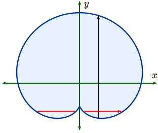
Example 3: The region $D$ that is shown to the right is Type I but is not Type II. Fixing $x$ and integrating first with respect to $y$ along the black line makes good sense because then $$ D \ = \ \Bigl\{\,(x,\,y) : \phi(x) \le y \le \psi(x),\ \ a \le x \le b\,\Bigl\}$$ for suitable choices of $a,\, b$ and functions $\phi(x),\, \psi(x)$: $$ \int \int_D\, f(x,\,y)\, dxdy = \int_a^b \left(\int_{\phi(x)}^{\psi(x)}\, f(x,\,y)\, dy\right) dx\,.$$ But if we had chosen to fix $y$, then the integral with respect to $x$ would sometimes split into two parts

shown in red. Not a good idea!

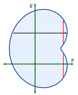
Example 4: The region $D$, shown to the right, is Type II but not Type I. Fixing $y$ and integrating first with respect to $x$ along the black line makes good sense because then $$ D \ = \ \Bigl\{\,(x,\,y) : \phi(y) \le x \le \psi(y),\ \ c \le y \le d\,\Bigl\}$$ for suitable choices of $c,\, d$ and functions $\phi(y),\, \psi(y)$. In this case $$ \int \int_D\, f(x,\,y)\, dxdy = \int_c^d \left(\int_{\phi(y)}^{\psi(y)}\, f(x,\,y)\, dx\right) dy\,.$$ But if we had chosen to fix $x$, then the integral with respect to $y$ would sometimes splits into two parts as shown in red. Again not a good idea!