Mappings in 2 dimensions

Changing variables is a very useful technique for simplifying many types of math problems. You can use a horizontal translation $f(x) \, \to\, f(x+1)$ to change a parabola $y = f(x) = x^2 - 2x + 1$ with vertex at the $(1,0)$ into another parabola $y = f(x+1) = x^2$ with vertex at the origin. We also use changes of variables to convert hard integrals into easier integrals. The change-of-variables formula for ordinary integrals is $$ \int_a^b\, f(x)\, dx \ = \ \int_{\alpha}^{\beta}\, f\big(g(u)\big)g'(u)\, du\,, \qquad g : [\alpha,\, \beta] \ \to \ [ a,\,b]\,.$$

Transformations in higher dimensions, called maps or mappings, play an even more important role in multi-variable calculus. We have already seen one such mapping ${\bf \Phi} : {\mathbb R}^2\,\to\, {\mathbb R}^2$, namely polar coordinates: $${\bf \Phi}: (r,\, \theta)\, \to\, (x,\, y)\,, \qquad x \ = \ r\cos \theta\,, \quad y \ = \ r\sin \theta\,,$$

The reason mappings like these are so useful in double integrals comes from their action on particular sets in the plane.

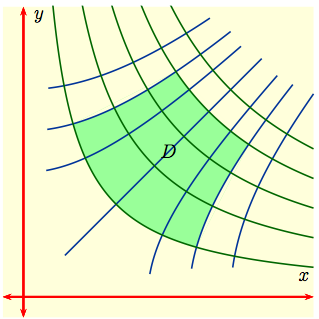
Let's start with a general double integral $$I \ = \ \int \int_D \,\, f(x, \,y)\, dx dy$$ over the green domain of integration $D$ in the $xy$-plane to the right. For such a $D$ finding the limits of integration might well be algebraically complicated, or the integration would be algebraically difficult, or both would be. Experience has shown that the integration would probably be much easier if $D$ were replaced by a rectangle with sides parallel to the coordinate axes.

  A mapping ${\bf \Phi} : {\mathbb R}^2\,\to\, {\mathbb R}^2$ and a rectangle $D^*$ with sides parallel to the axes in the $uv$-plane such that: $${\bf \Phi}(u,\, v) \ = \ (x(u,\,v),\, y(u,\,v))\,, \qquad {\bf \Phi}\big(D^*\big) \ = \ D\,;$$

  A 'distortion' function $\displaystyle{\frac{\partial(x,\,y)}{\partial(u,\,v)}}$ to replace $g'(u)$ so that $$ \int\int_D \, f(x,\, y)\, dxdy \ = \ \int\int_{D^*}\, f\big({\bf \Phi}(u,\,v)\big)\, \left|\frac{\partial(x,\,y)}{\partial(u,\,v)}\right|\,dudv\,.$$

In this case, if $D^* = [a,\,b]\times[c,\,d]$, then $$ \int\int_D \, f(x,\, y)\, dxdy \ = \ \int_a^b \left(\int_c^d \, f\big({\bf \Phi}(u,\,v)\big)\, \left|\frac{\partial(x,\,y)}{\partial(u,\,v)}\right|\,dv\right)du\,.$$

When the region of integration $D$ in the $xy$ plane has rotational symmetry, polar coordinates often send a rectangle $D^*$ in the $r\,\theta$ plane to a more complicated region $D$.

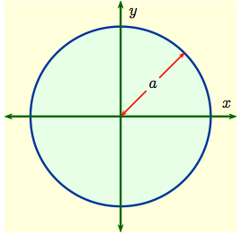
Example 1: When $D$ is a disk of radius $a$ centered at the origin, as shown to the right, then in $(x,\, y)$-coordinates $$D \ = \ \bigl\{ (x,\,y) : x^2 + y^2 \ \le \ a^2\,\bigl\}\,.$$ On the other hand, in the $r\theta$-plane $$D^* \ = \ \bigl\{ (r,\,\theta) : 0 \le r \le a,\ \ 0 \le \theta \le 2 \pi\,\bigl\}$$ is a rectangle.

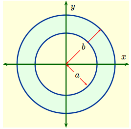
Example 2: When $D$ is an annulus centered at the origin between circles of radius $a,\, b, \ \ a < b$ as shown to the right, then in $(x,\, y)$-coordinates $$D \ = \ \bigl\{ (x,\,y) : a^2 \le x^2 + y^2 \ \le \ b^2\,\bigl\}\,.$$ On the other hand, in the $r\theta$-plane $$D^* \ = \ \bigl\{ (r,\,\theta) : a \le r \le b,\ \ 0 \le \theta \le 2 \pi\,\bigl\}$$ is a rectangle.