Examples

The following video demonstrates ways to use the change-of-variable formula to simplify integrals. In it, we compute the integral of $e^{x+2y}$ over a parallelogram, and the integral of $x^2$ over an off-center ellipse.

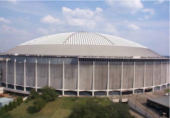
Example 1: Let's illustrate this change of variable idea in the case of polar coordinates. The Astrodome in Houston as shown to the right below might be modelled mathematically as the region below the cap of a sphere

$$ x^2+y^2+z^2 \ = \ R^2$$ above a circular disk $$ D = \{(x,\,y) : x^2 + y^2 \le a^2\}\,.$$ In terms of double integrals its $$ \hbox{Volume} \ = \ \int\int_D\, \sqrt{R^2 - x^2 - y^2}\, dx dy\,.$$ Rotational symmetry suggests changing to polar coordinates!

The Astrodome problem showed how this works when ${\bf \Phi}$ is the change of coordinates from polar to Cartesian coordinates, but matrix mappings often help too. They usually come in two 'flavors' as indicated in

Example 2a: Use the transformation $${\bf \Phi} : (u,\, v) \ \longrightarrow \ \bigl(\,x(u,\, v),\ y(u,\, v)\, \bigr)$$ with $$x \ = \ \frac{1}{2}\bigl(u-v\bigl) \,, \quad y \ = \ \frac{1}{2}\bigl(u+v\bigl) $$ to evaluate the integral $$ I \ = \ \int\int_D\ (x+y) \, dx dy$$ when $D$ is the square shown to the right.

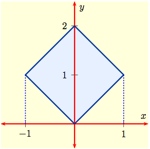
Example 2b: Use an appropriate transformation $${\bf \Phi} : (u,\, v) \ \longrightarrow \ \bigl(\,x(u,\, v),\ y(u,\, v)\, \bigr)$$ to evaluate the integral $$ I \ = \ \int\int_D\ (x+y) \, dx dy$$ when $D$ is the square having corner points $$(0,\,0)\,, \ \ (1,\, 1)\,, \ \ (0,\, 2)\,, \ \ (-1,\, 1)\,.$$ as shown to the right.

Solution for Example 2a: When $$x \ = \ \frac{1}{2}\bigl(u-v\bigl) \,, \quad y \ = \ \frac{1}{2}\bigl(u+v\bigl) $$ the Jacobian of the transformation $${\bf \Phi} : (u,\, v) \ \longrightarrow \ \bigl(\,x(u,\, v),\ y(u,\, v)\, \bigr)$$ is given by $$\frac{\partial (x,\,y)}{\partial (u,\,v)} \ = \ \left|\begin{matrix} \displaystyle {\frac{1}{2}}& \displaystyle{-\frac{1}{2}}\cr \\ \displaystyle {\frac{1}{2}}& \displaystyle { \frac{1}{2}}\end{matrix}\right|\ = \ \frac{1}{2}\,.$$ On the other hand, $$x+y \ = \ \frac{1}{2}\bigl(u-v\bigl) + \frac{1}{2}\bigl(u+v\bigl)\ = \ u\,.$$ So if ${\bf \Phi}$ maps $D^*$ onto $D$, then $$I \ = \ \frac{1}{2}\int_a^b\int_c^d\ u\ du dv\,.$$

It remains to find $a,\, b,\, c,\,d$ knowing that $${\bf \Phi}(a,\,c)\,=\, (0,\,0)\,, \quad {\bf \Phi}(b,\,c)\,=\, (1,\,1)$$ $${\bf \Phi}(b,\,d)\,=\, (0,\,2)\,, \quad {\bf \Phi}(a,\,d)\,=\, (-1,\,1)$$ But $x,\, y$ is given in terms of $u,\, v$: $$2x \ = \ u-v \,, \quad 2y \ = \ u+v\,, $$ so we need to solve for $u,\,v$: $$u\ = \ x+y \,, \qquad v\ = \ y-x\,.$$ This shows that $$a \,=\, c\,=\, 0, \quad b\,=\, 2, \quad d\,=\, 2\,,$$ Consequently, $$I \ = \ \frac{1}{2}\int_0^2\int_0^2\ u\, dudv\ = \ 2\, .$$

Solution for Example 2b: Since we know the corners of $D$, we can use the point slope formula to express $D$ as the square enclosed by the pairs of parallel lines $$y=x,\ \ y= x+2, \quad y=-x,\ \ y=-x +2\,.$$ Thus $D$ is the region $$\big\{ (x,\,y) : 0 \le x+y \le 2,\ \ 0 \le y -x \le 2\big\}$$ in the $xy$-plane. This suggests setting $$ u \,=\, x+y,\quad v\,=\, y-x\,,$$ $$ D^* \ = \ \big\{ (u,\,v) : 0\le u \le 2,\ 0 \le v \le 2\big\}\,.$$

To determine $${\bf \Phi} : (u,\, v) \to (x(u,\,v),\, v(u,\, v))$$ we need to express $x,\, y$ in terms of $u,\, v$. Solve for $x,\,y$ in the earlier linear equations: $$x \ = \ \frac{1}{2}\bigl(u-v\bigl) \,, \quad y \ = \ \frac{1}{2}\bigl(u+v\bigl) \,.$$ Consequently, after calculating the Jacobian as before we get $$I \ = \ \frac{1}{2}\int_0^2\int_0^2\ u\, dudv\ = \ 2\, .$$