Jacobians

The distortion factor between size in $uv$-space and size in $xy$ space is called the Jacobian. The following video explains what the Jacobian is, how it accounts for distortion, and how it appears in the change-of-variable formula.

Definition: The Jacobian of the transformation $${\bf \Phi}: (u,\,v) \ \longrightarrow \ (x(u,\, v), \, y(u, \,v))$$ is the $2\, \times\, 2$ determinant $$\frac{\partial (x,\,y)}{\partial (u, \,v)} \ = \ \left|\,\begin{matrix}\displaystyle { \frac{\partial x}{\partial u}} & \displaystyle { \frac{\partial x}{\partial v} } \cr \\ \displaystyle { \frac{\partial y}{\partial u} }& \displaystyle { \frac{\partial y}{\partial v}} \end{matrix}\,\right|\,.$$

Change-of-variable formula: If a 1-1 mapping $\Phi$ sends a region $D^*$ in $uv$-space to a region $D$ in $xy$-space, then $$\iint_D f(x,y) dx\,dy \ = \ \iint_{D^*} f(\Phi(u,v)) \left | \frac{\partial(x,y)} {\partial(u,v)} \right | du\, dv. $$ Note that this involves the absolute value of the Jacobian.

Example 1: Compute the Jacobian of the polar coordinates transformation $$x \ = \ r \cos \theta,\, \qquad y = r \sin \theta\,.$$ Solution: Since \begin{eqnarray*} & \frac{\partial x}{\partial r} = \cos(\theta), \quad & \frac{\partial y}{\partial r} = \sin(\theta), \\ & \frac{\partial x}{\partial \theta} = -r \sin(\theta), \quad & \frac{\partial y}{\partial \theta} = r \cos(\theta), \end{eqnarray*}

our Jacobian is $$ \left|\begin{matrix} \displaystyle { \frac{\partial x}{\partial r} }& \displaystyle{\frac{\partial x}{\partial \theta} }\cr \\ \displaystyle { \frac{\partial y}{\partial r} }& \displaystyle { \frac{\partial y}{\partial \theta}} \end{matrix}\right|\ = \ \left|\begin{matrix} \cos \theta & -r\sin \theta \cr \\ \sin \theta & r \cos \theta \end{matrix}\right|\ = \ r\,.$$ This explains why there's an $r$ factor in polar integrals! The area element $dA=dx\,dy$ is not equal to $dr\,d\theta$. Instead, $dA$ is equal to $r\, dr\,d\theta$.

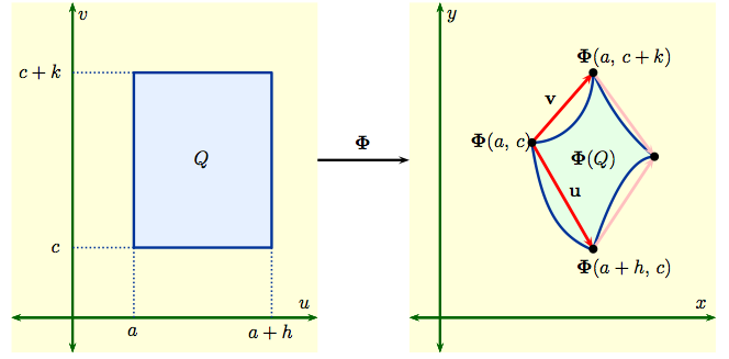
Then $${\bf u} \ = \ {\bf \Phi}(a+h,\,c) - {\bf \Phi}(a,\,c)\,, \qquad {\bf v} \ = \ {\bf \Phi}(a,\,c+k) - {\bf \Phi}(a,\,c)\,.$$ The area of the parallelogram spanned by ${\bf u} = u_1 {\bf i} + u_2 {\bf j}$ and ${\bf v} = v_1 {\bf i} + v_2 {\bf j}$ is the determinant $\left | \begin{matrix} u_1 & v_1 \cr u_2 & v_2 \end{matrix}\right |$.

Since $\hbox{area}(Q) \, =\, hk$, this means that the area of our region in the $xy$ plane is given by the absolute value of the Jacobian times the area in the $uv$ plane. Our shorthand for this is $$dA \ = \ dx\, dy \ = \ \left | \frac{\partial(x,y)}{\partial(u,v)} \right | du \, dv.$$

Areas are always positive, so the area of a small parallelogram in $xy$-space is always the absolute value of the Jacobian times the area of the corresponding rectangle in $uv$-space.

So why didn't we see an absolute value in the change-of-variables formula in one dimension? This had to do with the way we write the limits of integration.

Example 2: Compute $\int_0^{10} e^{-x/5} dx$. Solution: We did this before using $x=g(u)=5u$. Instead, let's take $x=-5u$, so $g'(u)=-5$ is negative. Now $e^{-x/5}=e^u$ and $dx= -5 du$. The map $g$ sends the interval from 0 to -2 in $u$-space to the interval from 0 to 10 in $x$-space, and our change-of-variable formula says $$\int_0^{10} e^{-x/5} dx \ = \ \int_0^{-2} -5 e^{u} du.$$ Of course, we usually integrate from $-2$ to $0$, not from $0$ to $-2$.

Flipping the limits of integration changes the sign of the answer, so $$\int_0^{10} e^{-x/5} dx \ = \ \int_{-2}^{0} +5 e^{u} du = 5(1-e^{-2}).$$ If we had written our 1-dimensional integrals in terms of regions instead in terms of starting points and end points, we would have had a factor of $+5$, rather than $-5$, all along. The mapping $x=-5u$ sends the region $D^*=[-2,0]$ to the region $D=[0,10]$, and $$\int_D e^{-x/5} dx \ = \ \int_{D^*} e^u \left | \frac{dx}{du} \right| du.$$