Geometry of Partial Derivatives

Home

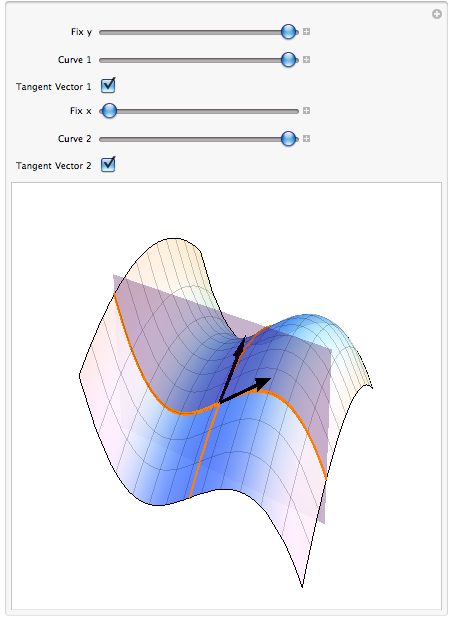
To understand partial derivatives geometrically, we need to interpret the algebraic idea of fixing all but one variable geometrically. This is equivalent to slicing a surface by a plane to produce a curve in space.

Start with the surface $$z \ = \ f(x,\, y) \ = \ 3x^2 -y^2 -x^3 +2,$$ shown to the right. Then $$f_x \ = \ \frac{\partial f}{\partial x} \ = \ \frac{\partial } {\partial x}\, \bigl( 3x^2 -y^2 -x^3 +2\bigl) \ = \ 6x -3x^2 \,.$$ To understand what this means, fix a value of $y$, say $y=-1$. Equivalently, slice the surface $z=f(x,y)$ with the plane $y=-1$, as in the figure. The cubic curve of intersection is shown in orange and can be given the parametrization $${\bf r}(x)\, = \, \bigl\langle\, x,\, -1,\, f(x,\,-1)\,\bigl\rangle\,=\, \bigl\langle\, x,\, -1,\, 3x^2 -x^3 +1\,\bigl\rangle\,.$$ A vector tangent to this orange curve is $${\bf r}'(x)\ = \ \bigl\langle\, 1,\, 0,\, 6x -3x^2\,\bigl\rangle \ = \ \bigl\langle\, 1,\, 0,\, f_x\,\bigl\rangle\,,$$ Thus $f_x$ gives the slope of the surface $z = f(x,\,y)$ as we move in the $x$-direction.

Likewise, if we fix $x= 1$, we see that $f_y$ gives the slope of the other orange curve (obtained by intersecting our surface with the plane $x=1$) as we move in the $y$-direction. Thus

At a point $P=(a,\,b,\, f(a,\,b))$ on the graph of $z = f(x,\, y)$,

The value $\displaystyle\frac{\partial f}{\partial x}\Bigl|_{(a,\,b)}$ is the Slope in the $x$-direction,

$\displaystyle \Bigl\langle \, 1,\, 0,\, \frac{\partial f}{\partial x}\Bigl|_{a,\,b}\,\Bigl \rangle$ is a Tangent Vector in the $x$-direction, while $$\frac{\partial f}{\partial y}\Bigl|_{(a,\,b)}\, \qquad \hbox{and} \qquad \Bigl\langle \, 0,\, 1,\, \frac{\partial f}{\partial y}\Bigl|_{a,\,b}\,\Bigl \rangle$$ give the slope and a tangent vector at $P$ in the $y$-direction.

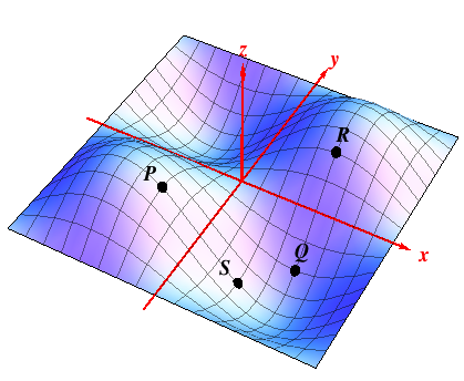
Example 1: Determine whether $f_x ,\ f_y$ are positive, negative, or zero at the points $P,\ Q, \ R,$ and $S$ on the surface to the right.
Solution: Starting at $Q$, the surface slopes up for fixed $x$ as $y$ increases, so $f_y\bigl|_{Q} > 0$, while moving slightly in the $x$ direction takes us neither uphill nor downhill, so so $f_x\bigl|_{Q}= 0$. Likewise, $$f_x\bigl|_{R} \,=\,0,\quad f_y\bigl|_{R} \,>\, 0\,, \qquad f_x\bigl|_{P} \,<\, 0,\, \quad f_y\bigl|_{P} \,=\, 0 \,.$$ We leave the signs of $f_x \bigl|_{S}$ and $f_y\bigl|_S$ to you.

All the same ideas carry over in exactly the same way to functions $f(x,\,y,\,z)$ of three or more variables - just don't expect lots of pictures!! The partial derivative $f_z$, for instance, is simply the derivative of $f(x,\,y,\,z)$ with respect to $z$, keeping the variables $x$ AND $y$ fixed now.

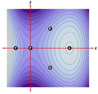
Information about the partial derivatives of a function $f(x,\,y)$ can be detected also from the contour map of $f$. Indeed, as one knows from using contour maps to learn whether a path on a mountain is going up or down, or how steep it is, so the sign of the partial derivatives of $f(x,\,y)$ and relative size can be read off from the contour map of $f$.

Example 2: To the right is the contour map of the earlier function $$f(x,\, y) \ = \ 3x^2 -y^2 -x^3 +2\,,$$ with 'higher ground' being shown in lighter colors and 'lower ground' in darker colors. Determine whether $f_x,\, f_y$ are positive, negative, or zero at $P,\, Q,\, R,\, S$, and $T$.

At $R$, the colors are lighter (higher) to the right and darker (lower) to the left, so $f_x \bigl |_R > 0$. Likewise, the colors are lighter below $R$ than above $R$, so $f_y \bigl |_R<0$. At $P$ and at $S$, the ground is flat: $S$ is at a local maximum, and $P$ is at a saddle. In both cases, $f_x=f_y=0$. We leave the remaining points to you.

Integration by Parts

Integrals of Trig Functions

Trig Substitutions

Partial Fractions

Strategies of Integration

Improper Integrals

Modeling with Differential Equations

Euler's Method and Direction Fields

Separable Equations

Models of Growth

Linear Equations

Parametrized Curves

Calculus with Parametrized Curves

Polar Coordinates

Areas and Lengths of Polar Curves

Conic sections

Conic Sections in Polar Coordinates

Infinite Sequences

Infinite Series

Integral Test

Comparison Tests

Convergence of Series with Negative Terms

The Ratio and Root Tests

Strategies for testing Series

Power Series

Representing Functions as Power Series

Taylor and Maclaurin Series

Applications of Taylor Polynomials

Functions of 2 and 3 variables

Partial Derivatives

Differentiability and the Chain Rule

Multiple Integrals

Iterated Integrals over Rectangles

Double Integrals over General Regions

Double integrals in polar coordinates

Multiple integrals in physics

Integrals in Probability and Statistics

Change of Variables