Jacobians

Home

The distortion factor between size in $uv$-space and size in $xy$ space is called the Jacobian. The following video explains what the Jacobian is, how it accounts for distortion, and how it appears in the change-of-variable formula.

Definition: The Jacobian of the transformation $${\bf \Phi}: (u,\,v) \ \longrightarrow \ (x(u,\, v), \, y(u, \,v))$$ is the $2\, \times\, 2$ determinant $$\frac{\partial (x,\,y)}{\partial (u, \,v)} \ = \ \left|\,\begin{matrix}\displaystyle { \frac{\partial x}{\partial u}} & \displaystyle { \frac{\partial x}{\partial v} } \cr \\ \displaystyle { \frac{\partial y}{\partial u} }& \displaystyle { \frac{\partial y}{\partial v}} \end{matrix}\,\right|\,\ = \ \frac{\partial x}{\partial u} \frac{\partial y}{\partial v} - \frac{\partial x}{\partial v}\frac{\partial y}{\partial u}.$$ Note that the bars around the $2 \times 2$ matrix mean ''determinant'', not absolute value. The Jacobian $\frac{\partial(x,y)}{\partial(u,v)}$ may be positive or negative.

Change-of-variable formula: If a 1-1 mapping $\Phi$ sends a region $D^*$ in $uv$-space to a region $D$ in $xy$-space, then $$\iint_D f(x,y) dx\,dy \ = \ \iint_{D^*} f(\Phi(u,v)) \left | \frac{\partial(x,y)} {\partial(u,v)} \right | du\, dv. $$ Note that this involves the absolute value of the Jacobian. Even when the Jacobian is negative, the distortion in volume is positive.

Example 1: Compute the Jacobian of the polar coordinates transformation $$x \ = \ r \cos \theta,\, \qquad y = r \sin \theta\,.$$ Solution: Since \begin{eqnarray*} & \frac{\partial x}{\partial r} = \cos(\theta), \quad & \frac{\partial y}{\partial r} = \sin(\theta), \\ & \frac{\partial x}{\partial \theta} = -r \sin(\theta), \quad & \frac{\partial y}{\partial \theta} = r \cos(\theta), \end{eqnarray*}

our Jacobian is $$ \left|\begin{matrix} \displaystyle { \frac{\partial x}{\partial r} }& \displaystyle{\frac{\partial x}{\partial \theta} }\cr \\ \displaystyle { \frac{\partial y}{\partial r} }& \displaystyle { \frac{\partial y}{\partial \theta}} \end{matrix}\right|\ = \ \left|\begin{matrix} \cos \theta & -r\sin \theta \cr \\ \sin \theta & r \cos \theta \end{matrix}\right|\ = \ r\,.$$ This explains why there's an $r$ factor in polar integrals! The area element $dA=dx\,dy$ is not equal to $dr\,d\theta$. Instead, $dA$ is equal to $r\, dr\,d\theta$.

Let's see why the Jacobian is the distortion factor in general for a mapping $${\bf \Phi} : (u,\, v) \ \to \ (x(u,\,v),\, y(u,\,v)) \ = \ x(u,\,v)\, {\bf i} +y(u,\,v)\, {\bf j}\,, $$ making good use of all the vector calculus we've developed so far. Let $Q = [a,\,a+h]\times [c,\,c+k]$ be a rectangle in the $uv$-plane and ${\bf \Phi}(Q)$ its image in the $xy$-plane as shown in

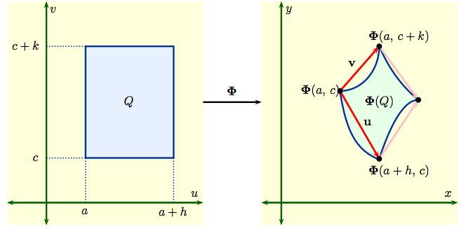
Then $${\bf u} \ = \ {\bf \Phi}(a+h,\,c) - {\bf \Phi}(a,\,c)\,, \qquad {\bf v} \ = \ {\bf \Phi}(a,\,c+k) - {\bf \Phi}(a,\,c)\,.$$ The area of the parallelogram spanned by ${\bf u} = u_1 {\bf i} + u_2 {\bf j}$ and ${\bf v} = v_1 {\bf i} + v_2 {\bf j}$ is the determinant $\left | \begin{matrix} u_1 & v_1 \cr u_2 & v_2 \end{matrix}\right |$.

By the definition of partial derivatives, $$\frac{{\bf \Phi}(a+h,\,c) - {\bf \Phi}(a,\,c)}{h} \ \approx \ \frac{\partial {\bf \Phi}}{\partial u}\Big|_{(a,c)}\ = \ \frac{\partial x}{\partial u}\Big|_{(a,c)}\, {\bf i} + \frac{\partial y}{\partial u}\Big|_{(a,c)}\, {\bf j} \,,$$ $$\frac{{\bf \Phi}(a,\,c+k) - {\bf \Phi}(a,\,c)}{k} \ \approx \ \frac{\partial {\bf \Phi}}{\partial v}\Big|_{(a,c)}\ = \ \frac{\partial x}{\partial v}\Big|_{(a,c)}\, {\bf i} + \frac{\partial y}{\partial v}\Big|_{(a,c)}\, {\bf j}\,.$$ We then compute $$\hbox{area}(\Phi(Q)) \approx \left | \begin{matrix} u_1 & v_1 \cr u_2 & v_2 \end{matrix}\right | \ \approx \ \left | \begin{matrix} h \frac{\partial x}{\partial u} & k \frac{\partial x}{\partial v} \cr h \frac{\partial y}{\partial u} & k \frac{\partial y}{\partial v} \end{matrix} \right | \ = \ hk \left | \begin{matrix} \frac{\partial x}{\partial u} & \frac{\partial x}{\partial v} \cr \frac{\partial y}{\partial u} & \frac{\partial y}{\partial v}\end{matrix} \right |. $$

Since $\hbox{area}(Q) \, =\, hk$, this means that the area of our region in the $xy$ plane is given by the absolute value of the Jacobian times the area in the $uv$ plane. Our shorthand for this is $$dA \ = \ dx\, dy \ = \ \left | \frac{\partial(x,y)}{\partial(u,v)} \right | du \, dv.$$

Areas are always positive, so the area of a small parallelogram in $xy$-space is always the absolute value of the Jacobian times the area of the corresponding rectangle in $uv$-space.

So why didn't we see an absolute value in the change-of-variables formula in one dimension? This had to do with the way we write the limits of integration.

Example 2: Compute $\int_0^{10} e^{-x/5} dx$.

Solution: We did this before using $x=g(u)=5u$. Instead, let's take $x=-5u$, so $g'(u)=-5$ is negative. Now $e^{-x/5}=e^u$ and $dx= -5 du$. The map $g$ sends the interval from 0 to -2 in $u$-space to the interval from 0 to 10 in $x$-space, and our change-of-variable formula says $$\int_0^{10} e^{-x/5} dx \ = \ \int_0^{-2} -5 e^{u} du.$$ Of course, we usually integrate from $-2$ to $0$, not from $0$ to $-2$.

Flipping the limits of integration changes the sign of the answer, so $$\int_0^{10} e^{-x/5} dx \ = \ \int_{-2}^{0} +5 e^{u} du = 5(1-e^{-2}).$$

If we had written our 1-dimensional integrals in terms of regions instead in terms of starting points and end points, we would have had a factor of $+5$, rather than $-5$, all along. The mapping $x=-5u$ sends the region $D^*=[-2,0]$ to the region $D=[0,10]$, and $$\int_D e^{-x/5} dx \ = \ \int_{D^*} e^u \left | \frac{dx}{du} \right| du.$$

Integration by Parts

Integrals of Trig Functions

Trig Substitutions

Partial Fractions

Strategies of Integration

Improper Integrals

Modeling with Differential Equations

Euler's Method and Direction Fields

Separable Equations

Models of Growth

Linear Equations

Parametrized Curves

Calculus with Parametrized Curves

Polar Coordinates

Areas and Lengths of Polar Curves

Conic sections

Conic Sections in Polar Coordinates

Infinite Sequences

Infinite Series

Integral Test

Comparison Tests

Convergence of Series with Negative Terms

The Ratio and Root Tests

Strategies for testing Series

Power Series

Representing Functions as Power Series

Taylor and Maclaurin Series

Applications of Taylor Polynomials

Functions of 2 and 3 variables

Partial Derivatives

Differentiability and the Chain Rule

Multiple Integrals

Iterated Integrals over Rectangles

Double Integrals over General Regions

Double integrals in polar coordinates

Multiple integrals in physics

Integrals in Probability and Statistics

Change of Variables