Visualizing Functions in 3 Dimensions

In this and the next few modules, we will be discussing functions of more than one variable.  Our familiar $y=f(x)$ is a curve in  2-dimensional space, with points $(x,y)$.  Now consider $z=f(x,y)$, which is a function of two (independent) variables, $x$ and $y$.  Here, $z$ is the value assigned to the function, which is unique given $x$ and $y$ (because $f$ is a function).  This function is a surface in 3-dimensional space, with points having coordinates $(x,y,z)$.   Similarly, $w=f(x,y,z)$ is a function of three variables, living in the very-difficult-to-see 4-dimensional space.  Much can be (and is) said to help you thoroughly understand these functions in a standard third-semester calculus course, but we are being brief here.  Our goal is to give you a quick introduction to the ideas of partial differentiation and multiple integration.

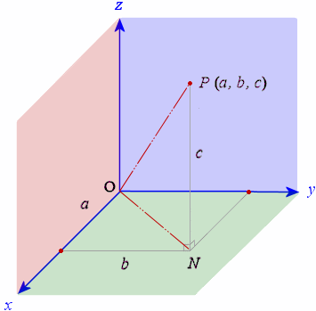
It can be challenging to see 3-space on the two dimensional page.  Think of this graphic as a room.  View the origin $O$ as being the back corner, so the back wall is purple, the left wall is pink, and the floor is green.  The point $(a,b,c)$ is $a$ units in the $x$-direction (along the $x$-axis toward the front of the room), $b$ units in the $y$-direction (to the right), and $c$-units in the $z$-direction (up).  Our earthly world is 3-dimensional space, and if oriented with an origin, all points in space have three coordinates. http://www.intmath.com/
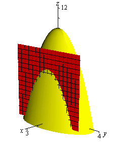
The function $z=f(x,y)$ can be represented in 3-space as a surface.  This yellow paraboloid is the surface given by the function $f(x,y)=10-4x^2-y^2$.  Notice that $f(0,0)=10$, giving the point $(0,0,10)$ on the surface.  Fixing $x=1$, we get a 2-dimensional slice (by the red slicer) of the surface, $z=6-y^2$, which is a parabola in the $yz$-plane, upside down (since the $y$ coefficient is negative) and shifted up by 6 units.  tutorial.math.lamar.edu
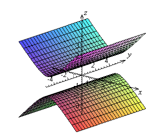
The graph here is of $z^2=1+x^2$.  Two things to notice.  First, this is not a function, since there is more than one value of $z$ for given values of $x$ and $y$.  (We have a vertical line test in this orientation of 3 dimensions, which this curve fails.)  We can represent this curve as two functions:  $f(x,y)=\sqrt{1+x^2}$ (the upper surface), and $g(x,y)=-\sqrt{1+x^2}$ (the lower surface).  The second thing we notice is that there is no $y$ in the formula, which means $y$ doesn't matter.  For example, $f(0,77)=f(0,-8)=f(0,\text{any number})=1$, and $g(0,46)=g(0,0)=g(0,\text{any number})=-1$.  Graphically, this means we get a line in the $y$-direction for any given $x$ and $z$ values.   www.engr.mun.ca

When you have trouble picturing "slices" when we take derivatives, etc., refer back to these graphs.  You are not expected to be able to graph such functions in this course, but when you are trying to visualize how we take partial derivatives, understanding points on and slices of surfaces will be very helpful.