Iterated Integrals over Rectangles

In order to integrate over a rectangle $[a,b] \times [c,d]$ , we first integrate with respect to one variable (say, $y$ ) for each fixed value of $x$ . That's an ordinary integral, which we can compute using the fundamental theorem of calculus. We then integrate the result over the other variable (in this case $x$ ), which we can also compute using the fundamental theorem of calculus. So a 2-dimensional double integral becomes two ordinary 1-dimensional integrals, one inside the other. We call this an iterated integral.

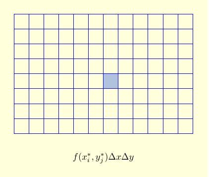
There are two ways to see the relation between double integrals and iterated integrals. In the bottom-up approach, we evaluate the sum

$\sum_{i=1}^m\sum_{j=1}^n f\left(x_{i}^*,y_{j}\right)^* \,\Delta x\,\Delta y=\sum_{i=1}^m \left(\sum_{j=1}^n f\left(x_{i}^*,y_{j}^*\right) \,\Delta x\,\right) \Delta y,$ by first summing over all of the boxes with a fixed

$i$ to get the contribution of a column (as indicated with the parentheses on the second sum), and then adding up the columns. (We could do this in the other order, by reversing the summations.)

$f\left(x_{i}^*,y_{j}^*\right)\, \Delta y\, \Delta x$ is the contribution of the volume of a tower over a single rectangle to our double integral, which approximates the volume under the surface $f(x,y) and over the rectangle.

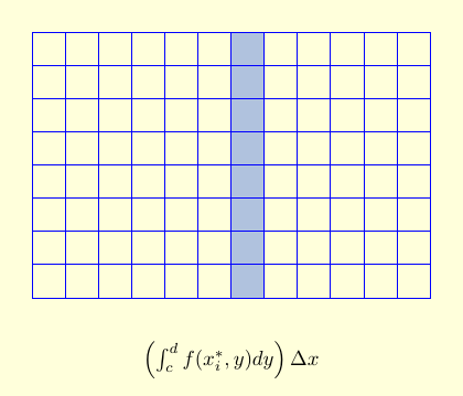
$\displaystyle\left(\sum_{j=1}^n f\left(x_{i}^*,y_{j}^*\right) \,\Delta y\,\right) \Delta x$ is the sum of volumes of towers over all the rectangles in a single column, approximating the volume under the surface over the column. Here,

$\Delta x$ is the width of the column. As

$n \to \infty$ , the sum over

$n$ turns into an integral, and we get

$\displaystyle\left (\int_c^d f\left(x, y\right)\,dy \right )\, \Delta x.$

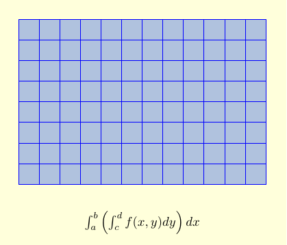
Adding up the columns then gives

$\displaystyle\sum_{i=1}^m \left (\int_c^d f\left(x_i^*, y\right)\, dy \right )\, \Delta x$ . Taking a limit as

$m \to \infty$ turns the sum into an iterated integral, giving us the actual volume over the large rectangle, under the surface:

$\int_a^b \left ( \int_c^d f(x,y)\, dy \right ) \,dx.$

This approach is explained in the following video, and an example is worked out. (Video Fix? However, there is a small error. At the beginning it says that we're going to integrate over the rectangle $[0,1] \times [0,2]$ , but for the rest of the video the region $R$ is actually the rectangle $[0,2] \times [0,1]$ .)

The Fundamental Theorem of Calculus

The Indefinite Integral and the Net Change

Substitution

Area Between Curves

Volumes

Integration by Parts

Integrals of Trig Functions

Trig Substitutions

Partial Fractions

Strategies of Integration

Improper Integrals

Differential Equations

Models of Growth

Infinite Sequences

Infinite Series

Integral Test

Comparison Tests

Convergence of Series with Negative Terms

The Ratio and Root Tests

Strategies for testing Series

Power Series

Representing Functions as Power Series

Taylor and Maclaurin Series

Applications of Taylor Polynomials

Partial Derivatives

Multiple Integrals

Iterated Integrals over Rectangles

Double Integrals over General Regions

How To Compute Iterated Integrals