Iterated Integrals over Rectangles

Home

One Variable at the Time

Now that we know what double integrals are, we can start to compute them. The key idea is: One variable at a time!

In order to integrate over a rectangle $[a,b] \times [c,d]$, we first integrate over one variable (say, $y$) for each fixed value of $x$. That's an ordinary integral, which we can do using the fundamental theorem of calculus. We then integrate the result over the other variable (in this case $x$), which we can also do using the fundamental theorem of calculus. So a 2-dimensional double integral boils down to two ordinary 1-dimensional integrals, one inside the other. We call this an iterated integral.

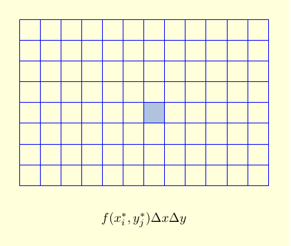
There are two ways to see the relation between double integrals and iterated integrals. In the bottom-up approach, we evaluate the sum $$\sum_{i=1}^m \sum_{j=1}^n f\left(x_{i}^*,y_{j}^*\right) \,\Delta x\, \Delta y,$$ by first summing over all of the boxes with a fixed $i$ to get the contribution of a column, and then adding up the columns. (Or we can sum over all of the boxes with a fixed $j$ to get the contribution of a row, and then add up the rows.)

$f\left(x_{i}^*,y_{j}^*\right)\, \Delta y\, \Delta x$ is the approximate contribution of a single box to our double integral.

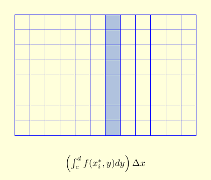
$\displaystyle\sum_{j=1}^n f\left(x_{i}^*,y_{j}^*\right) \,\Delta y\, \Delta x$ is the approximate contribution of all the boxes in a single column. As $n \to \infty$, the sum over $n$ turns into an integral, and we get $$\displaystyle\left (\int_c^d f\left(x_i^*, y\right)\,dy \right )\, \Delta x.$$

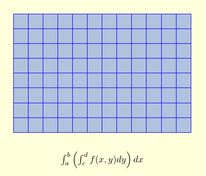
Adding up the columns then gives $\displaystyle\sum_{i=1}^m \left (\int_c^d f\left(x_i^*, y\right)\, dy \right )\, \Delta x$. Taking a limit as $m \to \infty$ turns the sum into an iterated integral: $$\int_a^b \left ( \int_c^d f(x,y)\, dy \right ) \,dx.$$

This bottom-up approach is explained in the following video. (Video Fix? However, there is a small error. At the beginning it says that we're going to integrate over the rectangle $[0,1] \times [0,2]$, but for the rest of the video the region $R$ is actually the rectangle $[0,2] \times [0,1]$.)

Cavalieri's Principle

An alternate approach to finding volumes (and hence double integrals) - the so-called Slice Method - was formulated by Cavalieri and is expressed mathematically in

Cavalieri's Principle: let $W$ be a solid and $P_x,\, a \le x \le b,$ be a family of parallel planes such that

$W$ lies between $P_a$ and $P_{\,b}$,
the area of the cross-sectional slice of $W$ cut by $P_x$ is $A(x)$.

Then $$\hbox{ volume of} \ W \ = \ \int_a^b\, A(x)\, dx\,.$$

We already used this idea to compute volumes of revolution. Suppose $W$ is created by rotating the graph of $y = f(x),\, a \le x \le b,$ about the $x$-axis. When $P_x$ is a plane perpendicular to the $x$-axis, then the slice of $W$ cut by $P_x$ is a disk of radius $f(x)$. Here $A(x) = \pi f(x)^2$, so we recover the familiar result $$\hbox{ volume of} \ W \ = \ \pi \int_a^b\, f(x)^2\, dx$$ for a volume of revolution. But Cavalieri's Principle does not require the cross-sections to be triangles or disks!

Example: Find the volume of the solid $W$ under the hyperbolic paraboloid $$z \ = \ f(x,\, y) \ = \ 2+ x^2 - y^2 $$ and over the square $D\,= \,[-1,\,1]\,\times\,[-1,\,1]$.

Solution: The solid is shown below.

When $P_x$ is the vertical slice perpendicular to the $x$-axis for fixed $x$ shown in purple, then $$A(x) =\int_{-1}^2\, (2+x^2 - y^2)\, dy\qquad \qquad$$ $$\qquad = \left[\,2y +x^2y -\frac{y^3}{3}\right]_{-1}^1= \frac{10}{3} +2x^2 \,.$$ But then by using the slider to fill out the solid, Cavalieri's Principle shows that $W$ has $$\hbox{volume} \ = \ \int_{-1}^1\, A(x)\, dx \ = \ \int_{-1}^1\, \left(\frac{10}{3} +2x^2\right)\,dx \ = \ \left[\frac{10x}{3} +\frac{2x^3}{3}\right]_{-1}^1 \ = \ 8\,.$$

In other words, the volume of a region is $\int_a^b A(x)\, dx$, where $A(x)$ is the cross-sectional area at a particular value of $x$. But that's the area under the curve $z=f(x,y)$, where we are treating $x$ as a constant and $y$ as our variable. That is,

The double integral $\displaystyle\iint_R f(x,y)\, dA$ equals the iterated integral $\displaystyle\int_a^b \left (\int_c^d f(x,y) \,dy\right )\, dx$.

The Fundamental Theorem of Calculus

The Indefinite Integral and the Net Change

Substitution

Area Between Curves

Volumes

Integration by Parts

Integrals of Trig Functions

Trig Substitutions

Partial Fractions

Strategies of Integration

Improper Integrals

Differential Equations

Models of Growth

Infinite Sequences

Infinite Series

Integral Test

Comparison Tests

Convergence of Series with Negative Terms

The Ratio and Root Tests

Strategies for testing Series

Power Series

Representing Functions as Power Series

Taylor and Maclaurin Series

Applications of Taylor Polynomials

Partial Derivatives

Multiple Integrals

Iterated Integrals over Rectangles

Double Integrals over General Regions

One Variable at the Time

Cavalieri's Principle